

aswath_damodaran-investment_philosophies_2012
.pdf100 |
|
|
|
INVESTMENT PHILOSOPHIES |
|||
|
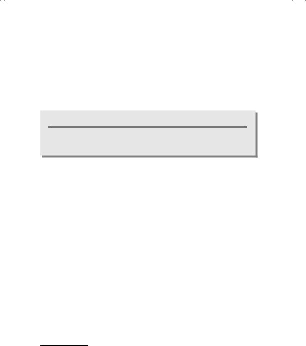
T A B L E 4 . 3 Value of Rental Building |
|
|
|
|||
|
|
|
|
|
|
|
|
|
Year |
Expected Cash Flows |
Value at End |
PV at 9.51% |
|||
|
|
|
|
|
|
|
|
1 |
$1,050,000 |
|
$ |
958,817 |
|
||
2 |
$1,102,500 |
|
$ |
919,329 |
|
||
3 |
$1,157,625 |
|
$ |
881,468 |
|
||
4 |
$1,215,506 |
|
$ |
845,166 |
|
||
5 |
$1,276,282 |
|
$ |
810,359 |
|
||
6 |
$1,340,096 |
|
$ |
776,986 |
|
||
7 |
$1,407,100 |
|
$ |
744,987 |
|
||
8 |
$1,477,455 |
|
$ |
714,306 |
|
||
9 |
$1,551,328 |
|
$ |
684,888 |
|
||
10 |
$1,628,895 |
|
$ |
656,682 |
|
||
11 |
$1,710,339 |
|
$ |
629,638 |
|
||
12 |
$1,795,856 |
$2,500,000 |
$ |
1,444,124 |
|
||
|
Value of building = |
|
$ |
10,066,749 |
|
||
To illustrate these principles, assume that you are trying to value a rental building for purchase. The building is assumed to have a finite life of 12 years and is expected to have cash flows before debt payments and after taxes of $1 million, growing at 5 percent a year for the next 12 years. The real estate is also expected to have a value of $2.5 million at the end of the 12th year (called the salvage value). Based on your costs of borrowing and the cost you attach to the equity you will have invested in the building, you estimate a cost of capital of 9.51 percent. The value of the building can be estimated in Table 4.3.
Note that the cash flows over the next 12 years represent a growing annuity, and the present value could have been computed with a simple present value equation, as well.
|
|
(1.05)12 |
|
|
|
|
|
1,000,000(1.05) 1 − |
|
|
|
|
|
Value of building = |
(1.0951)12 |
|
+ |
2,500,000 |
||
|
(0.0951 − 0.05) |
|
(1.0951)12 |
|||
= |
$10,066,749 |
|
|
|
|
|
This building has a value of $10.07 million.
V a l u i n g a n A s s e t w i t h a n I n f i n i t e L i f e
When we value businesses and firms, as opposed to individual assets, we are often looking at entities that have no finite lives. If they reinvest sufficient

Show Me the Money: The Basics of Valuation |
101 |
amounts in new assets each period, firms could keep generating cash flows forever. In this section, we value assets that have infinite lives and uncertain cash flows.
E q u i t y a n d F i r m V a l u a t i o n In the section on valuing assets with equity risk, we introduced the notions of cash flows to equity and cash flows to the firm. We argued that cash flows to equity are cash flows after debt payments, all expenses, and reinvestment needs have been met. In the context of a business, we will use the same definition to measure the cash flows to its equity investors. These cash flows, when discounted back at the cost of equity for the business, yield the value of the equity in the business. This is illustrated in Figure 4.6.
Note that our definition of both cash flows and discount rates is consistent—they are both defined in terms of the equity investor in the business.
There is an alternative approach in which, instead of valuing the equity stake in the asset or business, we look at the value of the entire business. To do this, we look at the collective cash flows not just to equity investors but also to lenders (or bondholders in the firm). The appropriate discount rate is the cost of capital, since it reflects both the cost of equity and the cost of debt. The process is illustrated in Figure 4.7.
Note again that we are defining both cash flows and discount rates consistently, to reflect the fact that we are valuing not just the equity portion of the investment but the investment itself.
D i v i d e n d s a n d E q u i t y V a l u a t i o n When valuing equity investments in publicly traded companies, you could argue that the only cash flows investors in these investments get from the firm are dividends. Therefore, the value
|
|
Assets |
|
Liabilities |
|
||
Cash flows considered |
Assets in Place |
Debt |
|||||
|
|
|
|
|
|||
are cash flows from assets, |
|
|
|
|
|
||
after debt payments and |
|
Discount rate reflects only the |
|||||
after making reinvestments |
|
||||||
needed for future growth. |
|
cost of raising equity financing. |
|||||
|
|
|
Growth Assets |
Equity |
|
|
|
|
|
|
|
||||
|
|
|
|
|
|
|
|
|
|
|
|
|
|
|
|
|
|
|
|
|
|
|
|
Present value is value of just the equity claims on the firm.
F I G U R E 4 . 6 Equity Valuation

102 |
|
|
|
INVESTMENT PHILOSOPHIES |
||
|
|
Assets |
|
Liabilities |
||
|
|
|||||
|
|
|
|
|
|
|
Cash flows considered |
Assets in Place |
Debt |
||||
are cash flows from assets, |
|
Discount rate reflects the cost |
||||
prior to any debt payments |
|
|||||
|
of raising both debt and equity |
|||||
but after firm has |
|
|||||
|
financing, in proportion to their |
|||||
reinvested to create |
|
|||||
|
use. |
|||||
growth assets. |
|
|||||
Growth Assets |
Equity |
|
||||
|
|
|
|
|
|
|
|
|
|
|
|
|
|
|
|
|
|
|
|
|
Present value is value of the entire firm, and reflects the value of all claims on the firm.
F I G U R E 4 . 7 Firm Valuation
of the equity in these investments can be computed as the present value of expected dividend payments on the equity.
t=∞
Value of equity (only dividends) =
E(Dividendt)
t=1 (1 + ke)t
The mechanics are similar to those involved in pricing a bond, with dividend payments replacing coupon payments, and the cost of equity replacing the interest rate on the bond. The fact that equity in a publicly traded firm has an infinite life, however, indicates that we cannot arrive at closure on the valuation without making additional assumptions.
One way in which we might be able to estimate the value of the equity in a firm is by assuming that the dividends, starting today, will grow at a constant rate forever. If we do that, we can estimate the value of the equity using the present value formula for a perpetually growing cash flow. In fact, the value of equity will be:
Value of equity (dividends growing at a constant rate forever)
=
E(Dividend next period)
(ke − gn)
This model, which is called the Gordon growth model, is simple but limited, since it can value only companies that pay dividends, and only if these dividends are expected to grow at a constant rate forever. The reason this is a restrictive assumption is that no asset or firm’s cash flows can grow forever at a rate higher than the growth rate of the economy. If it
Show Me the Money: The Basics of Valuation |
103 |
did, the firm would become the economy. Therefore, the constant growth rate is constrained to be less than or equal to the economy’s growth rate. For valuations of firms in U.S. dollars in 2012, this puts an upper limit on the growth rate of approximately 2 to 3 percent.4 This constraint will also ensure that the growth rate used in the model will be less than the discount rate.
N U M B E R W A T C H
Valuation of Consolidated Edison: See the spreadsheet that contains the valuation of Con Ed.
We will illustrate this model using Consolidated Edison, the utility that produces power for much of New York. Con Ed paid dividends per share of $2.40 in 2010. The dividends are expected to grow 2 percent a year in the long term, and the company has a cost of equity of 8 percent. The value per share can be estimated as follows:
Value of equity per share = $2.40(1.02)/(0.08 − 0.02) = $40.80
The stock was trading at $42 per share at the time of this valuation. We could argue that based on this valuation, the stock was mildly overvalued.
What happens if we have to value a stock whose dividends are growing at 15 percent a year? The solution is simple. We value the stock in two parts. In the first part, we estimate the expected dividends each period for as long as the growth rate of this firm’s dividends remains higher than the growth rate of the economy, and sum up the present value of the dividends. In the second part, we assume that the growth rate in dividends will drop to a stable or constant rate forever sometime in the future. Once we make this assumption, we can apply the Gordon growth model to estimate the
4The nominal growth rate of the U.S. economy through the 1990s was about 5 percent. The growth rate of the global economy, in nominal U.S. dollar terms, has been about 6 percent over that period. In the last decade, growth has slowed. A good proxy for long-term nominal growth is the risk-free rate, which has dropped to about 2% in both the United States and in Europe.
104 |
INVESTMENT PHILOSOPHIES |
present value of all dividends in stable growth. This present value is called the terminal price and represents the expected value of the stock in the future, when the firm becomes a stable-growth firm. The present value of this terminal price is added to the present value of the dividends to obtain the value of the stock today.
t=N
Value of equity with high-growth dividends =
E(Dividendst)
t=1 (1 + ke)t
+ Terminal priceN (1 + ke)N
where N is the number of years of high growth and the terminal price is based on the assumption of stable growth beyond year N.
Terminal price = E(DividendN+1) (ke − gn)
N U M B E R W A T C H
Valuation of Procter & Gamble: See the spreadsheet that contains the valuation of P&G.
To illustrate this model, assume that you were trying to value Procter & Gamble (P&G), one the leading consumer product companies in the world, owning some of the most valuable brands, including Gillette razors, Pampers diapers, Tide detergent, Crest toothpaste, and Vicks cough medicine. P&G reported earnings per share of $3.82 in 2010 and paid out 50 percent of these earnings as dividends that year. We will use a beta of 0.90, reflecting the beta of large consumer product companies in 2010, a risk-free rate of 3.50 percent, and a mature market equity risk premium of 5 percent to estimate the cost of equity:
Cost of equity = 3.50% + 0.90(5%) = 8.00%
We estimated a 10 percent growth rate, in conjunction with earnings and dividends for the next five years, and discounting these dividends back

Show Me the Money: The Basics of Valuation |
105 |
at the cost of equity, we arrive at a cumulative value of $10.09 per share for the dividends during these five years:
|
1 |
2 |
3 |
4 |
5 |
Sum |
|
|
|
|
|
|
|
Earnings per share |
$4.20 |
$4.62 |
$5.08 |
$5.59 |
$6.15 |
|
Payout ratio |
50.00% |
50.00% |
50.00% |
50.00% |
50.00% |
|
Dividends per share |
$2.10 |
$2.31 |
$2.54 |
$2.80 |
$3.08 |
|
Cost of equity |
8.00% |
8.00% |
8.00% |
8.00% |
8.00% |
|
Present value |
$1.95 |
$1.98 |
$2.02 |
$2.06 |
$2.09 |
$10.09 |
|
|
|
|
|
|
|
After year 5, we assume that P&G will be in stable growth, growing 3 percent a year (just below the risk-free rate). To go with the lower growth, we assume that the firm would pay out 75 percent of its earnings as dividends and face a slightly higher cost of equity of 8.5 percent.5
Value per share at end of year 5 = EPS5(1 + Growth rateStable)(Payout ratioStable) (Cost of equityStable − Growth rateStable)
= $6.15(1.03)(0.75) = $86.41 (0.085 − 0.03)
Discounting this price to the present at 8 percent (the cost of equity for the high-growth period) and adding to the present value of expected dividends during the high-growth period yields a value per share of $68.90.
Value per share = PV of dividends in high growth
+ PV of value at end of high growth
$86.41 = $10.09 + 1.085 = $68.90
The stock was trading at $68 in May 2011, making it fairly valued.6
A B r o a d e r M e a s u r e o f C a s h F l o w s t o E q u i t y There are two significant problems with the use of just dividends to value equity. The first is that it
5Costs of equity generally go down in stable growth, but this case is an exception. P&G is a below-average risk company during high growth. We expect it to become an average risk firm during stable growth.
6A. Damodaran, Investment Valuation, 3rd ed. (Hoboken, NJ: John Wiley & Sons, 2012).

106 |
INVESTMENT PHILOSOPHIES |
works only if cash flows to the equity investors take the form of dividends. It will not work for valuing equity in private businesses, where the owners often withdraw cash from the business but may not call it dividends, and it may not even work for publicly traded companies if they return cash to the equity investors by buying back stock, for instance. The second problem is that the use of dividends is based on the assumption that firms pay out what they can afford to in dividends. When this is not true, the dividend discount models will misestimate the value of equity, under estimating value when they pay too little and over estimating value when they pay too much.
To counter this problem, we come up a broader definition of cash flow that we call free cash flow to equity, defined as the cash left over after operating expenses, interest expenses, net debt payments, and reinvestment needs. Reinvestment needs include investments in both long-term assets and short-term assets, with the former measured as the difference between capital expenditures and depreciation (net cap ex) and the latter by the change in noncash working capital. By net debt payments, we are referring to the difference between new debt issued and repayments of old debt. If the new debt issued exceeds debt repayments, the free cash flow to equity will be higher.
Free cash flow to equity (FCFE) = Net income − Reinvestment needs − (Debt repaid − New debt issued)
Think of this as potential dividends, or what the company could have paid out in dividends. To illustrate, in 2010, Coca-Cola reported net income of $11,809 million, capital expenditures of $2,215 million, depreciation of $1,443 million, and an increase in noncash working capital of $335 million. Incorporating the fact that Coca-Cola raised $150 million more in debt than it repaid, we can compute the free cash flow to equity as follows:
FCFECoca-Cola = Net income − (Cap ex − Depreciation)
−Change in noncash working capital
−(Debt repaid − New debt raised)
=11,809 − (2,215 − 1,443) − 335 − (−150)
=$10.852 million
The difference between the net income and the FCFE represents the portion of net income reinvested back by equity investors in Coca-Cola in 2010.
Equity reinvestment = Net income − FCFE = $11,809 − $10,852 = $957 million
Show Me the Money: The Basics of Valuation |
107 |
Coca-Cola paid out about $6 billion in dividends during the year, well below its free cash flow to equity. Consequently, using the dividend discount model would understate the value of equity in Coca-Cola.
N U M B E R W A T C H
Valuation of Coca-Cola: See the spreadsheet that contains the valuation of Coca-Cola.
Once the free cash flows to equity have been estimated, the process of estimating value parallels the dividend discount model. To value equity in a firm where the free cash flows to equity are growing at a constant rate forever, we use the present value equation to estimate the value of cash flows in perpetual growth:
Value of equity in infinite-life asset = E(FCFE1) (ke − gn)
All the constraints relating to the magnitude of the constant growth rate used that we discussed in the context of the dividend discount model continue to apply here.
In the more general case, where free cash flows to equity are growing at a rate higher than the growth rate of the economy, the value of the equity can be estimated again in two parts. The first part is the present value of the free cash flows to equity during the high growth phase, and the second part is the present value of the terminal value of equity, estimated based on the assumption that the firm will reach stable growth sometime in the future.
t=N
Value of equity with high-growth FCFE =
E(FCFEt)
t=1 (1 + ke)t
+ Terminal value of equityN (1 + ke)N
With the FCFE approach, we have the flexibility we need to value equity in any type of business or publicly traded company. Applying this approach to Coca-Cola in 2010, we assumed that Coca-Cola’s net income would grow 7.5 percent a year for the next five years and that it would reinvest 25 percent of its net income each year back into the business. In addition, we assumed

108 |
|
|
INVESTMENT PHILOSOPHIES |
||
T A B L E 4 . 4 Expected Cash Flows and Value Today |
|
|
|||
|
|
|
|
|
|
Sum |
1 |
2 |
3 |
4 |
5 |
|
|
|
|
|
|
Expected growth rate |
7.50% |
7.50% |
7.50% |
7.50% |
7.50% |
Net income |
$12,581 |
$13,525 |
$14,539 |
$15,630 |
$16,802 |
Equity reinvestment rate |
25.00% |
25.00% |
25.00% |
25.00% |
25.00% |
FCFE |
$9,436 |
$10,144 |
$10,905 |
$11,722 |
$12,602 |
Cost of equity |
8.45% |
8.45% |
8.45% |
8.45% |
8.45% |
Cumulative cost of equity |
1.0845 |
1.1761 |
1.2755 |
1.3833 |
1.5002 |
Present value |
$8,701 |
$8,625 |
$8,549 |
$8,474 |
$8,400 |
|
|
|
|
|
|
that the cost of equity for Coca-Cola during this five-year period would be 8.45 percent. The resulting FCFE and the present value of these cash flows is shown in Table 4.4.
The sum of the present values of the FCFE for the next five years is $42,749 million. At the end of year 5, we assumed that Coca-Cola would be in stable growth, growing 3 percent a year, reinvesting 20 percent of its net income back into the business, with a cost of equity of 9 percent. The value of equity at the end of year 5 can then be computed:
Value of equity at end of year 10
= Expected net income in year 5(1 + gstable)(1 − Equity reinvestment ratestable) (Stable cost of equity − gstable)
= $16,802(1.03)(0.80) = $230,750 million (0.09 − 0.03)
Discounting the terminal value back at the cumulated cost of equity for year 5 and adding to the present value of FCFE over the next 5 years yields an overall value for equity from operating assets.
Value of equity today = PV of FCFE + PV of terminal value
=$42,749 + $230,750/1.5002
=$196,562 million
Dividing by the number of shares outstanding (2,289.25 million) yields a value per share of $85.86, well above the prevailing stock price of $68.22 at the time of the valuation.
F r o m V a l u i n g E q u i t y t o V a l u i n g t h e F i r m A firm is more than just its equity investors. It has other claim holders, including bondholders and banks.

Show Me the Money: The Basics of Valuation |
109 |
When we value the firm, therefore, we consider cash flows to all of these claim holders. We define the free cash flow to the firm as being the cash flow left over after operating expenses, taxes, and reinvestment needs, but before any debt payments (interest or principal payments).
Free cash flow to firm (FCFF) = After-tax operating income − Reinvestment needs
The two differences between FCFE and FCFF become clearer when we compare their definitions. The free cash flow to equity begins with net income, which is after interest expenses and taxes, whereas the free cash flow to the firm begins with after-tax operating income, which is before interest expenses. Another difference is that the FCFE is after net debt payments, whereas the FCFF is before net debt payments.
What exactly does the free cash flow to the firm measure? One interpretation is that it measures the cash flows generated by the assets before any financing costs are considered and thus is a measure of operating cash flow. Another read of it is that the free cash flow to the firm is the cash flow used to service all claim holders’ needs for cash—interest and principal to debt holders and dividends and stock buybacks to equity investors.
To illustrate the estimation of free cash flow to the firm, consider Toyota in 2010. In that year, Toyota reported operating income of 933 billion yen, had a tax rate of 40 percent, and reinvested 112 billion yen in new investments (net capital expenditures and working capital). The free cash flow to the firm for Toyota in 2010 is then:
FCFFBoeing = Operating income (1 − Tax rate) − Reinvestment needs = 933(1 − 0.40) − 112 = 448 billion yen
Note that the tax computed is a hypothetical tax, i.e., the tax that Toyota would have paid, if they had been taxed on their entire operating income.7 Once the free cash flows to the firm have been estimated, the process of computing value follows a familiar path. If valuing a firm or business with free cash flows growing at a constant rate forever, we can use the perpetual growth equation:
Value of firm with FCFF growing at constant rate = E(FCFF1) (kc − gn)
7We don’t count the tax benefits from interest expenses in the cash flows because it is counted in the cost of capital, through the use of an after-tax cost of debt.