218M. Herant and M. Dembo

Because of the multiphase nature of the flow (one has to solve the triplet vn , vs, and P rather than just for v and P), this last step requires some modifications from the usual treatment.

By adding the solvent and network momentum equation (Eq. 10.5 and 10.6) together, vs can be eliminated to obtain a “bulk” cytoplasmic momentum equation:

This is to be complemented with the appropriate boundary condition for stress across the membrane, which, in usual situations, looks like

where Pext is the external pressure, γ and κ the surface tension and mean curvature. The solvent momentum equation (Eq. 10.5) gives an expression for vs :

which can then be substituted in the incompressibility condition to yield:

In situations where there is zero membrane permeability (in other words, no transmembrane solvent flow) the boundary condition simplifies to:

Following the standard Uzawa method, an initial guess for the pressure field allows the computation of the network velocity field by Eq. 10.24. This velocity field can then be used to update the pressure field by Eq. 10.27, and so on through iterations between the two equations. Once the network velocity field vn and pressure field P have converged to a self-consistent solution, the solvent velocity field vs can be trivially extracted through the use of Eq. 10.26 with automatic enforcement of the incompressibility condition.

An example of cellular protrusion

Probably the simplest possible case of cellular protrusion is the emergence of a single pseudopod from an isolated, initially round nonadherent cell. This configuration has the advantages of a simple geometry with two-dimensional cylindrical symmetry and of avoiding potential confounding factors that appear when the mechanics of adhesion is involved. The formation of such pseudopods has been studied in individual neutrophils by Zhelev et al. (2004) and modeled in some detail by Herant et al. (2003). Here we present a simplified version of this process as a pedagogical introduction to the basic principles that are involved.

We will describe behaviors under both a cytoskeleton-membrane-repulsion and cytoskeleton-swelling model. In both cases, we make the following assumptions:

Initial condition is that of a round cell of diameter 8.5 µm.

Cortical tension is γ = 0.025 dyn cm−1.

Equilibrium network (cytoskeleton) volume fraction is θ0 = 0.1% (Watts and Howard 1993) everywhere inside the cell except:

Network fraction over a spherical patch of cell surface (diameter 1 µm) is fixed to one percent.

Away from the frontal patch, network fraction evolves to its equilibrium

according to first order kinetics with time-scale τn = 20 seconds, that is dθn /dt = (θ0 − θn )/τn .

Network viscosity is given by ν0θn where ν0 = 6 × 106 poise so that the baseline interior viscosity of the cell is ν = ν0θ0 = 6000 poise.

These values are reasonable approximations of the characteristics of human neutrophils (see Herant et al., 2003).

The idea is that in both the repulsion and the swelling models, the excess cytoskeleton at the activated patch of cortex will drive the formation of a pseudopod. Bracing by the viscous interior of the cell allows outward protrusion against the restoring force of the cortical tension that tends to sphericize the cell.

Protrusion driven by membrane–cytoskeleton repulsion

The mechanics of membrane–cytoskeleton repulsion as a driver of protrusion is straightforward as follows: (i) a region with increased cytoskeletal density appears due to enhanced polymerization at the leading edge of the pseudopod. (ii) Due to repulsion from the cortical membrane, cytoskeleton flows into the cell while cytosol is sucked forward. (iii) Cytoskeletal flow into the cell is opposed by viscous resistance of the underlying cytoplasm. By action and reaction, this leads to bulging out of the membrane, eventually creating and lengthening a pseudopod.

As has been pointed out, the quantity that matters for the dynamics of membrane– cytoskeleton interaction is the product of the membrane–cytoskeleton interaction stress density M with the range δ of the interaction. In numerical simulations that encompass the whole cell, it is not practical to try to accurately model the details of the cytoskeletal dynamics near the membrane as depicted in Fig. 10-2. Instead, the stress contribution to the network momentum equation (Eq. 10.6) is integrated over the range δ of network–membrane interaction. So, if we allow a generous average of 6 kB T interaction energy per actin monomer within range of the membrane, we have

where n is the unit normal vector to the membrane. If we would like the pseudopod to extend a few µm within about a minute, we need the flow velocity of cytoskeleton to be of order 0.2 µm s−1. By Eqs. 10.17 and 10.29, this means that δ 0.5 µm.

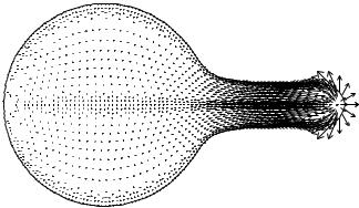
Fig. 10-5 shows the outline of the cell together with the network velocity field sixty seconds into a two-dimensional cylindrical symmetry simulation starting from a round cell. The flow clearly changes direction right at the pseudopod surface with the disjoining membrane–cytoskeleton force driving out the membrane while causing a centripetal flow of cytoskeleton into the cell.

The observant reader has probably noted that in this simulation, the frontal surface of the pseudopod has a curiously uniform velocity. This is because the additional

220 M. Herant and M. Dembo

Fig. 10-5. Simulation Protrusion driven by membrane – cytoskeleton repulsion. Length of the pseudopod is 6 µm, pseudopod velocities are 0.1 µm s−1.

velocity constraint of “no-shear” was introduced at the tip of the pseudopod. In the absence of such a prescription, membrane–network repulsion can drive severe rippling instabilities whereby the membrane grows folds that rapidly lengthen in a way reminiscent of the Rayleigh-Taylor instability (heavy over light fluid). From a biological point of view, the “no-shear” condition that we had to impose could point to rigid transverse cross-linking of filaments at the leading edge that prevent sliding. This instability also provides a potential mechanism for the formation of microvilli.

Protrusion driven by cytoskeletal swelling

The mechanics of cytoskeletal swelling as a driver of protrusion is similar to that of cytoskeletal–membrane repulsion. A region with increased cytoskeletal density appears due to enhanced polymerization in a compartment close to the leading edge of the pseudopod. Under repulsive self-interaction, the dense clump of cytoskeleton swells, drawing in cytosol like an expanding sponge draws water. This is the volume flow that accounts for the growth of the pseudopod. Finally, expansion into the cell is balanced by viscous resistance of the underlying cytoplasm. This braces outward expansion, which – while it does not have to work against viscosity of an external medium (assumed to be inviscid) – does have to work against cortical tension as new cellular area is created by the growth of the pseudopod.

Following the discussion of network swelling and in parallel with the simulation of cytoskeletal–membrane repulsion, we assume a contribution of 6 kB T per actin monomer to the cytoskeletal swelling stress density

Fig. 10-6 shows the outline of the cell together with the network velocity field sixty seconds into the simulation, starting from a round cell. As in the simulation of protrusion driven by cytoskeletal–membrane repulsion, there is an obvious

Fig. 10-6. Protrusion driven by cytoskeletal swelling. Length of the pseudopod is 6 µm, pseudopod velocities are 0.1 µm s−1.

retrograde flow of cytoskeleton. However, one will note that the center of expansion is slightly behind the leading edge, so that there also exists a small region of forward cytoskeletal flow at the front of the pseudopod. This is in contrast with protrusion from cytoskeletal–membrane repulsion where the flow of cytoskeleton is retrograde all the way to the tip of the pseudopod and then changes to forward motion at the membrane. (In reality, this occurs at the “gap” region depicted in Fig. 10-2.)

Discussion

It is reassuring that choices of physico-biological parameters (such as viscosity or interaction energies) that seem by and large reasonable can lead to a plausible mechanism for the protrusion of a pseudopod. The morphology and extension velocity of the pseudopod is within range of the experimental data obtained for the neutrophil (Zhelev et al., 1996). In addition, retrograde flow similar to that observed in lamellipodial protrusion (for example, see Theriot and Mitchison, 1992) is evident. There are, however, some difficulties with each model. In the case of the membrane– cytoskeleton repulsion model, the range of interaction had to be set to 0.5 µm to obtain sufficient elongation velocity. This is a large distance compared to a monomer, but small compared to the persistence length of a filament (for instance, see Kovar and Pollard, 2004) which implies that the stress field would most likely have to be stored in the large scale strain energy from deformation of the cytoskeleton (Herant et al., 2006). In the case of the swelling model, it is difficult to build up clumps of cytoskeleton of significant density and size (as are observed) without prompt smoothing and dissipation by expansion. Although none of those caveats are model killers in the sense that more complicated explanations can be invoked to rescue them, they hint at more mechanical complexity than is presented in the rather simple approach followed here.

A separate but nonetheless important issue is that of discrimination between models. As Figs. 10-5 and 10-6 make clear, each model can produce a similar pseudopod.