210M. Herant and M. Dembo

Network–membrane interactions

The basic idea behind a network–membrane disjoining stress is that there exists a repulsive force between actin monomers (polymerized or unpolymerized) and the cortical membrane. For free (G-actin) subunits this has no dynamical consequences, as redistribution occurs freely in the cytosol. However, once subunits are sequestered into the cytoskeleton by polymerization, the repulsive force has dynamical consequences because it endows the cytoskeleton with a macroscopic stress. In other words, while free monomers cannot push back against the membrane, filaments can because they are braced by the entire inner cytoskeletal scaffolding of the cell (these concepts first came to the fore with the work of Hill and Kirschner, 1982).

To put these notions on a more formal footing, let us postulate a mean-field repulsive force between monomers (free or in a filament) and the cortical membrane that derives

from the interaction potential ψ M (r) where r is the distance from the membrane and where we set the constant by requiring limr→∞ ψ M (r) = 0. From equilibrium thermodynamics, we can relate the ratio of free monomer concentration far away ([Mfree(∞)]) and at distance r with the interaction potential as a Boltzmann factor:

Here we can think of ψ M (r) as the average work required to bring a monomer from infinity to distance r from the membrane.

At the same time we have the chemical reaction between the polymerized and unpolymerized state of the monomer.

Taking actin as an example where addition of free monomers into polymers occurs at the barbed ends of filaments, there exists a critical free-monomer density [Mcritfree] above which reaction 10.12 is driven to the right and below which it is driven to the left.

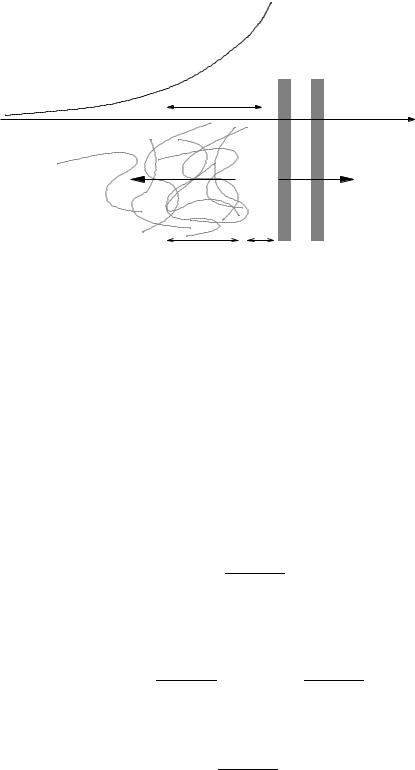
We need to examine 10.12 in the light of 10.11. Let us assume that the membrane– monomer interaction potential ψ M (r) decreases monotonously with distance from the membrane, and further that it is infinite (or very large) at zero distance from the membrane (see Fig. 10-2; in other words, the monomer is excluded from the membrane by a hard-core potential). Then it should be clear that in a region near the membrane, [Mfree(r)] is smaller than [Mcritfree], and hence that there cannot be any monomers added into polymers in this region. This region is labeled the ‘gap’ in Fig. 10-2. Advected polymers may appear in the gap, but unless they are stabilized by capping, they will tend to disassemble.

Further away from the membrane, ψ M (r) decreases to the point that [Mfree(r)] is smaller than [Mcritfree] and this allows the elongation of polymers by driving free monomers from the free to the bound state. Assuming that the polymerization of free monomers is rapid, we then have a region where [Mfree(r)] [Mcritfree]. This means that for the region of interest, that is, where polymerization is allowed to take place

(outside the gap) but within the region where membrane–monomer interaction is still

212M. Herant and M. Dembo

Natural logarithms of even very large numbers are seldom more than 10, and maximal volume fractions of cytoskeleton are 2% (see Hartwig and Shevlin, 1986). The

maximum disjoining stress at the membrane/cytoskeleton interface is thus of order 105 dyn cm−2 (104 Pa, 100 cm H2O).

Network dynamics near the membrane

One should be cautious not to assimilate the force-per-unit area of membrane or stress given in Eq. 10.16 to a protrusive force; in general the net outward force at the membrane as could theoretically be measured with a constraining spring would be considerably less. There are two reasons for this.

1.Imperfect cytoskeletal bracing against backflow: unless there exists some sort of mechanism to brace the cytoskeleton near the membrane, it will simply slide back, negating any outward force. In general, such bracing is expected to be provided by the viscoelastic properties of the cytoskeleton interior to the boundary layer, which transports stress to whatever is bracing the cell (in other words, the substratum).

2.Imperfect cytoskeletal decoupling from the membrane: if the cytoskeleton is somehow anchored to the membrane and cannot flow back, the stress FM is simply carried by the anchors and no outward force results.

We will assume here that the second condition is appropriately fulfilled, although experimental evidence is sometimes contradictory (for example, Listeria actin tails are attached to the Listeria, Gerbal et al., 2000). Let us further assume that the counteracting force to rear flow is provided by interior cytoskeletal viscosity. In that case, simple dimensional analysis (which can be made more rigorous, see Herant et al., 2003) gives

where ν is the viscosity and v is the velocity change near the membrane (see Fig. 10-2). In the case of perfect bracing and no external opposing force, the protrusive velocity is then v, but in the general case it will be less. In the limit of a stalled protrusion, the protrusive velocity is zero while the retrograde flow of cytoskeleton is − v. Note that within this picture, the important parameter is not the magnitude of M but rather its product with the range of the membrane–network interaction

M δ.

Finally, an interesting finding is that, if one assumes that the constitutive laws for the viscosity and for the network–membrane force have the same dependence on the cytoskeletal concentration, for example ν = ν0θn , M 0M θn , then one notices that Eq. 10.17 implies that v is independent of the network concentration near the membrane. Using numerical values for ν0 (6 × 106 poise, see Herant et al., 2003) and 0M (upper limit 5 × 106 dyn cm−2, see Eq. 10.16), one gets v < δ s−1. Typical velocities v at the leading edge are at least 10 nm s−1 and may range to as high as 0.5 µm s−1, (see Theriot and Mitchison 1992), which means that δ, the characteristic range of interaction, must be greater than 10 nm and even reach 0.5 µm.