

The cytoskeleton as a soft glassy material |
51 |
remodeling events reflecting their spatio-temporal reorganization (Fredberg, Jones et al., 1996). As discussed in Chapter 2, probes are now available that can measure each of these features with temporal resolution in the range of milliseconds and spatial resolution in the range of nanometers. Using such probes, this chapter demonstrates that a variety of phenomena that have been taken as the signature of condensed systems in the glassy state are prominently expressed by the cytoskeletal lattice of the living adherent cell. While highly specific interactions play out on the molecular scale, and homogeneous behavior results on the integrative scale, evidence points to metastability of interactions and nonequilibrium cooperative transitions on the mesoscale as being central factors linking integrative cellular function to underlying molecular events. Insofar as such fundamental functions of the cell – including embryonic development, contraction, wound healing, crawling, metastasis, and invasion – all stem from underlying cytoskeletal dynamics, identification of those dynamics as being glassy would appear to set these functions into an interesting context.
The chapter begins with a brief summary of experimental findings in living cells. These findings are described in terms of a remarkably simple empirical relationship that appears to capture the essence of the data with very few parameters. Finally, we show that this empirical relationship is predicted from the theory of soft glassy rheology (SGR). As such, SGR offers an intriguing perspective on mechanical behavior of the cytoskeleton and its relationship to the dynamics of protein-protein interactions.
Experimental findings in living cells
To study the rheology of cytoskeletal polymers requires a probe whose operative frequency range spans, insofar as possible, the internal molecular time scales of the rate processes in question. The expectation from such measurements is that the rheological behavior changes at characteristic relaxation frequencies, which in turn can be interpreted as the signature of underlying molecular interactions that dominate the response (Hill, 1965; Kawai and Brandt, 1980). Much of what follows in this chapter is an attempt to explain the failure to find such characteristic relaxation times in most cell types. The experimental findings of our laboratory, summarized below, are derived from single cell measurements using magnetic twisting cytometry (MTC) with optical detection of bead motion. Using this method, we were able to apply probing frequencies ranging from 0.01 Hz to 1 kHz. As shown by supporting evidence, these findings are not peculiar to the method; rather they are consistent with those obtained using different methods such as atomic force microscopy (Alcaraz, Buscemi et al., 2003).
Magnetic Twisting Cytometry (MTC)
The MTC device is a microrheometer in which the cell is sheared between a plate at the cell base (the cell culture dish upon which the cell is adherent) and a magnetic microsphere partially embedded into the cell surface, as shown in Fig. 3-1. We use ferrimagnetic microbeads (4.5 µm diameter) that are coated with a panel of antibody and nonantibody ligands that allow them to bind to specific receptors on the cell surface
52 |
J. Fredberg and B. Fabry |
|
|
|
|
|
|
|
(c) |
|
|
|
|
twisting field |
|
|
|
|
rotation |
|
|
|
|
cell |
|
1 m |
|
10 m |
displacement |
|
|
|
|
|
|
(a) |
(b) |
|
(d) |
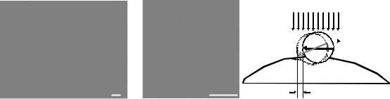
Fig. 3-1. (a) Scanning EM of a bead bound to the surface of a human airway smooth muscle cell.
(b)Ferrimagnetic beads coated with an RGD-containing peptide bind avidly to the actin cytoskeleton (stained with fluorescently labeled phalloidin) of HASM cells via cell adhesion molecules (integrins).
(c)A magnetic twisting field introduces a torque that causes the bead to rotate and to displace. Large arrows indicate the direction of the bead’s magnetic moment before (black) and after (gray) twisting. If the twisting field is varied sinusoidally in time, then the microbead wobbles to and fro, resulting in a lateral displacement, (d), that can be measured. From Fabry, Maksym et al., 2003.
(including various integrin subtypes, scavenger receptors, urokinase receptors, and immune receptors). The beads are magnetized horizontally by a brief and strong magnetic pulse, and then twisted vertically by an external homogeneous magnetic field that varies sinusoidally in time. This applied field creates a torque that causes the beads to rotate toward alignment with the field, like a compass needle aligning with the earth’s magnetic field. This rotation is impeded, however, by mechanical forces that develop within the cell as the bead rotates. Lateral bead displacements during bead rotation in response to the resulting oscillatory torque are detected by a CCD camera mounted on an inverted microscope.
Cell elasticity (g ) and friction (g ) can then be deduced from the magnitude and phase of the lateral bead displacements relative to the torque (Fig. 3-2). Image acquisition with short exposure times of 0.1 ms is phase-locked to the twisting field so that 16 images are acquired during each twisting cycle. Heterodyning (a stroboscopic technique) is used at twisting frequencies >1 Hz up to frequencies of 1000 Hz. The images are analyzed using an intensity-weighted center-of-mass algorithm in which sub-pixel arithmetic allows the determination of bead position with an accuracy of 5 nm (rms).
Measurements of cell mechanics
The mechanical torque of the bead is proportional to the external magnetic field (which was generated using an electromagnet), the bead’s magnetic moment (which was calibrated by measuring the speed of bead rotation in a viscous medium), and the cosine between the bead’s magnetization direction with the direction of the twisting field. Consider the specific torque of a bead, T , which is the mechanical torque per bead volume, and has dimensions of stress (Pa). The ratio of the complex-specific
˜ ˜
torque T to the resulting complex bead displacement d (evaluated at the twisting frequency) then defines a complex modulus of the cell g˜ = T˜/d˜, and has dimensions of
The cytoskeleton as a soft glassy material
(a)
[Pa/Gauss]T |
50 |
|
|
|
|
25 |
|
|
|
|
|
|
|
|
|
|
|
|
0 |
|
|
|
|
|
-25 |
|
|
|
|
|
-50 |
|
|
|
|
|
0 |
1 |
2 |
3 |
4 |
(b) |
|
|
time [s] |
|
|
400 |
|
|
|
|
|
|
|
|
|
0.01 Hz |
|
|
300 |
|
|
|
|
|
|
|
|
|
|
|
200 |
|
|
|
0.03 Hz |
|
100 |
|
|
|
0.1 Hz |
[nm] |
|
|
|
0.75 Hz |
|
0 |
|
|
|
1000 Hz |
|
|
|
|
|
|
10 Hz |
d |
-100 |
|
|
|
|
|
|
|
|
|
|
|
-200 |
|
|
|
|
|
-300 |
|
|
|
|
|
-400 |
|
|
|
|
|
-50 |
-25 |
0 |
25 |
50 |
|
|
|
T [Pa] |
|
|
53
250 |
|
125 |
[nm] |
0 |
|
|
d |
-125 |
|
-250 |
|
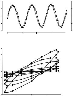
Fig. 3-2. (a) Specific torque T (solid line) and lateral displacement d (filled circles connected by a solid line) vs. time in a representative bead measured at a twisting frequency of 0.75 Hz. Bead displacement followed the sinusoidal torque with a small phase lag. The filled circles indicate when the image and data acquisition was triggered, which was 16 times per twisting cycle. (b) Loops of maximum lateral bead displacement vs. specific torque of a representative bead at different frequencies. With increasing frequency, displacement amplitude decreased. From Fabry, Maksym et al., 2003.
Pa/nm. These measurements can be transformed into traditional elastic shear (G ) and loss (G ) moduli by multiplication of g and g with a geometric factor that depends on the shape and thickness of the cell and the degree of bead embedding. Finite element analysis of cell deformation for a representative bead-cell geometry (assuming homogeneous and isotropic elastic properties with 10 percent of the bead diameter embedded in a cell 5 µm high) sets this geometric factor to 6.8 µm (Mijailovich, Kojic et al., 2002). This geometric factor need serve only as a rough approximation, however, because it cancels out in the scaling procedure described below, which is model independent. For each bead we compute the elastic modulus g (the real part of g˜), the loss modulus g (the imaginary part of g˜), and the loss tangent η (the ratio g /g ) at a given twisting frequency. These measurements are then repeated over a range of frequencies.
Because only synchronous bead movements that occur at the twisting frequency are considered, nonsynchronous noise is suppressed by this analysis. Also suppressed are higher harmonics of the bead motion that may result from nonlinear material properties and that – if not properly accounted for – could distort the frequency dependence of the measured responses. However, we found no evidence of nonlinear

54 J. Fredberg and B. Fabry
g [Pa/nm]
0.6
0.5  g'
g'
0.4
0.3
0.2
 g"
g"
0.1
0
0 |
50 |
100 |
150 |
|
|
T [Pa] |
|
Fig. 3-3. g and g vs. specific torque amplitude T . g and g were measured in 537 HASM cells at f = 0.75 Hz. Specific torque amplitudes T varied from 1.8 to 130 Pa. g and g were nearly constant, implying linear mechanical behavior of the cells in this range. Error bars indicate one standard error. From Fabry, Maksym et al., 2003.
cell behavior (such as strain hardening or shear thinning) at the level of stresses we apply with this technique, which ranges from about 1 Pa to about 130 Pa (Fig. 3-3). Throughout that range, which represents the physiological range, responses were linear.
Frequency dependence of g and g
The relationship of G and G vs. frequency for human airway smooth muscle (HASM) cells under control conditions is shown in Fig. 3-4, where each data point represents the median value of 256 cells. Throughout the frequency range studied, G increased with increasing frequency, f, according to a power law, f x−1 (as explained below, the formula is written in this way because the parameter x takes on a special meaning, namely, that of an effective temperature). Because the axes in Fig. 3-4 are logarithmic, a power-law dependency appears as a straight line with slope x − 1. The power-law exponent of G was 0.20 (x = 1.20), indicating only a weak dependency of G on frequency. G was smaller than G at all frequencies except at 1 kHz. Like G , G also followed a weak power law with nearly the same exponent at low frequencies. At frequencies larger than 10 Hz, however, G exhibited a progressively stronger frequency dependence, approaching but never quite attaining a power-law exponent of 1, which would be characteristic of a Newtonian viscosity.
This behavior was at first disappointing because no characteristic time scale was evident; we were unable to identify a dominating relaxation process. The only characteristic time scale that falls out of the data is that associated with curvilinearity of the G data that becomes apparent in the neighborhood of 100 Hz (Fig. 3-4). As shown below, this curvilinearity is attributable to a small additive Newtonian viscosity that is entirely uncoupled from cytoskeletal dynamics. This additive viscosity is on the order of 1 Pa s, or about 1000-fold higher than that of water, and contributes to the energy dissipation (or friction) only above 100 Hz. Below 100 Hz, friction (G ) remained a