Kluwer - Handbook of Biomedical Image Analysis Vol

volume data. The level set segmentation method, which is well documented in the literature [5–8], creates a new volume from the input data by solving an initial value partial differential equation (PDE) with user-defined feature-extracting terms. Given the local/global nature of these terms, proper initialization of the level set algorithm is extremely important. Thus, level set deformations alone are not sufficient, they must be combined with powerful initialization techniques in order to produce successful segmentations. Our level set segmentation approach consists of defining a set of suitable preprocessing techniques for initialization and selecting/tuning different feature-extracting terms in the level set algorithm. We demonstrate that combining several preprocessing steps, data analysis and level set deformations produce a powerful toolkit that can be applied, under the guidance of a user, to segment a wide variety of volumetric data.

There are more sophisticated strategies for isolating meaningful 3D structures in volume data. Indeed, the so-called segmentation problem constitutes a significant fraction of the literature in image processing, computer vision, and medical image analysis. For instance, statistical approaches [9–12] typically attempt to identify tissue types, voxel by voxel, using a collection of measurements at each voxel. Such strategies are best suited to problems where the data is inherently multivalued or where there is sufficient prior knowledge [13] about the shape or intensity characteristics of the relevant anatomy. Alternatively, anatomical structures can be isolated by grouping voxels based on local image properties. Traditionally, image processing has relied on collections of edges, i.e. high-contrast boundaries, to distinguish regions of different types [14–16]. Furthermore deformable models, incorporating different degrees of domainspecific knowledge, can be fitted to the 3D input data [17, 18].

This chapter describes a level set segmentation framework, as well as the the preprocessing and data analysis techniques needed to segment a diverse set of biological volume datasets. Several standard volume processing algorithms have been incorporated into framework for segmenting conventional datasets generated from MRI, CT, and TEM scans. A technique based on moving least-squares has been developed for segmenting multiple nonuniform scans of a single object. New scalar measures have been defined for extracting structures from diffusion tensor MRI scans. Finally, a direct approach to the segmentation of incomplete tomographic data using density parameter estimation is described. These techniques, combined with level set surface deformations, allow us to segment many different types of biological volume datasets.

8.2 Level Set Surface Models

When considering deformable models for segmenting 3D volume data, one is faced with a choice from a variety of surface representations, including triangle meshes [19, 20], superquadrics [21–23], and many others [18, 24–29]. Another option is an implicit level set model, which specifies the surface as a level set of a scalar volumetric function, φ : U →( IR, where U IR3 is the range of the surface model. Thus, a surface S is

with an isovalue k. In other words, S is the set of points s in IR3 that composes the kth isosurface of φ. The embedding φ can be specified as a regular sampling on a rectilinear grid.

Our overall scheme for segmentation is largely based on the ideas of Osher et al. [30] that model propagating surfaces with (time-varying) curvaturedependent speeds. The surfaces are viewed as a specific level set of a higher dimensional function φ—hence the name level set methods. These methods provide the mathematical and numerical mechanisms for computing surface deformations as isovalues of φ by solving a partial differential equation on the 3D grid. That is, the level set formulation provides a set of numerical methods that describes how to manipulate the grayscale values in a volume, so that the isosurfaces of φ move in a prescribed manner (shown in Fig. 8.1). This chapter does not present a comprehensive review of level set methods, but merely introduces the basic concepts and demonstrates how they may be applied to

Figure 8.1: (a) Level set models represent curves and surfaces implicitly using grayscale images. For example, an ellipse is represented as the level set of an image shown here. (b) To change the shape of the ellipse we modify the grayscale values of the image by solving a PDE.

418 Breen, Whitaker, Museth, and Zhukov

the problem of volume segmentation. For more details on level set methods see [7, 31].

There are two different approaches to defining a deformable surface from a level set of a volumetric function as described in Eq. (8.1). Either one can think of φ(s) as a static function and change the isovalue k(t) or alternatively fix k and let the volumetric function dynamically change in time, i.e. φ(s, t). Thus, we can mathematically express the static and dynamic models respecti-

To transform these definitions into partial differential equations which can be solved by standard numerical techniques, we differentiate both sides of Eq. (8.2) with respect to time t, and apply the chain rule:

The static equation (8.3a) defines a boundary value problem for the timeindependent volumetric function φ. This static level set approach has been solved [32, 33] using “Fast Marching Methods.” However, it inherently has some serious limitations following the simple definition in Eq. (8.2a). Since φ is a function (i.e. single-valued), isosurfaces cannot self-intersect over time, i.e. shapes defined in the static model are strictly expanding or contracting over time. However, the dynamic level set approach of eq. (8.3b) is much more flexible and shall serve as the basis of the segmentation scheme in this chapter. Equation (8.3b) is sometimes referred to as a “Hamilton–Jacobi-type” equation and defines an initial value problem for the time-dependent φ. Throughout the remainder of this chapter we shall, for simplicity, refer to this dynamical approach as the level set method, and not consider the static alternative.

Thus, to summarize the essence of the (dynamic) level set approach, let ds/dt be the movement of a point on a surface as it deforms, such that it can be expressed in terms of the position of s U and the geometry of the surface at that point, which is, in turn, a differential expression of the implicit function, φ.

dt

where F() is a user-created “speed” term that defines the speed of the level set at point s in the direction of the local surface normal n at s. F() may depend on a variety of local and global measures including the order-n derivatives of

φ, Dnφ, evaluated at s, as well as other functions of s, n, φ, and external data. Because this relationship applies to every level set of φ, i.e. all values of k, this equation can be applied to all of U , and therefore the movements of all the level set surfaces embedded in φ can be calculated from Eq. (8.4).

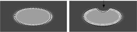
The level set representation has a number of practical and theoretical advantages over conventional surface models, especially in the context of deformation and segmentation. First, level set models are topologically flexible, they easily represent complicated surface shapes that can form holes, split to form multiple objects, or merge with other objects to form a single structure. These models can incorporate many (millions) degrees of freedom, and therefore they can accommodate complex shapes such as the dendrite in Fig. 8.7. Indeed, the shapes formed by the level sets of φ are restricted only by the resolution of the sampling. Thus, there is no need to reparameterize the model as it undergoes significant changes in shape.

The solutions to the partial differential equations described above are computed using finite differences on a discrete grid. The use of a grid and discrete time steps raises a number of numerical and computational issues that are important to the implementation. However, it is outside of the scope of this chapter to give a detailed mathematical description of such a numerical implementation. Rather we shall provide a summary in a later section and refer to the actual source code which is publicly available5.

Equation (8.4) can be solved using finite forward differences if one uses the up-wind scheme, proposed by Osher et al. [30], to compute the spatial derivatives. This up-wind scheme produces the motion of level set models over the entire range of the embedding, i.e., for all values of k in Eq. (8.2). However, this

5 The level set software used to produce the morphing results in this chapter is available for public use in the VISPACK libraries at http://www.cs.utah.edu/ whitaker/vispack.

method requires updating every voxel in the volume for each iteration, which means that the computation time increases as a function of the volume, rather than the surface area, of the model. Because segmentation requires only a single model, the calculation of solutions over the entire range of isovalues is an unnecessary computational burden.

This problem can be avoided by the use of narrow-band methods, which compute solutions only in a narrow band of voxels that surround the level set of interest [34, 35]. In a previous work [36] we described an alternative numerical algorithm, called the sparse-field method, that computes the geometry of only a small subset of points in the range and requires a fraction of the computation time required by previous algorithms. We have shown two advantages to this method. The first is a significant improvement in computation times. The second is increased accuracy when fitting models to forcing functions that are defined to subvoxel accuracy.

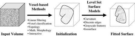
8.3 Segmentation Framework

The level set segmentation process has two major stages, initialization and level set surface deformation, as shown in Fig. 8.2. Each stage is equally important for generating a correct segmentation. Within our framework a variety of core operations are available in each stage. A user must “mix-and-match” these operations in order to produce the desired result [37]. Later sections describe specialized operations for solving specific segmentation problems that build upon and extend the framework.

Figure 8.2: Level set segmentation stages—initialization and surface

deformation.

8.3.1 Initialization

Because level set models move using gradient descent, they seek local solutions, and therefore the results are strongly dependent on the initialization, i.e., the starting position of the surface. Thus, one controls the nature of the solution by specifying an initial model from which the surface deformation process proceeds. We have implemented both computational (i.e. “semi-automated”) and manual/interactive initialization schemes that may be combined to produce reasonable initial estimates directly from the input data.

Linear filtering: We can filter the input data with a low-pass filter (e.g. Gaussian kernel) to blur the data and thereby reduce noise. This tends to distort shapes, but the initialization need only be approximate.

Voxel classification: We can classify pixels based on the filtered values of the input data. For grayscale images, such as those used in this chapter, the classification is equivalent to high and low thresholding operations. These operations are usually accurate to only voxel resolution (see [12] for alternatives), but the deformation process will achieve subvoxel results.

Topological/logical operations: This is the set of basic voxel operations that takes into account position and connectivity. It includes unions or intersections of voxel sets to create better initializations. These logical operations can also incorporate user-defined primitives. Topological operations consist of connected-component analyses (e.g. flood fill) to remove small pieces or holes from objects.

Morphological filtering: This includes binary and grayscale morphological operators on the initial voxel set. For the results in the chapter we implement openings and closings using morphological propagators [38,39] implemented with level set surface models. This involves defining offset surfaces of φ by expanding/contracting a surface according to the following PDE,

up to a certain time t. The value of t controls the offset distance from the original surface of φ(t = 0). A dilation of size α, Dα , corresponds to the solution of Eq. (8.5) at t = α using the positive sign, and likewise erosion, Eα , uses the negative sign. One can now define a morphological opening operator

ward specific features in the data. One must choose those properties of the input data to which the model will be attracted and what role the shape of the model will have in the deformation process. Typically, the deformation process combines a data term with a smoothing term, which prevents the solution from fitting too closely to noise-corrupted data. There are a variety of surface-motion terms that can be used in succession or simultaneously, in a linear combination to form F(x) in Eq. (8.4).

Curvature: This is the smoothing term. For the work presented here we use the mean curvature of the isosurface H to produce

The mean curvature is also the normal variation of the surface area (i.e., minimal surface area). There are a variety of options for second-order smoothing terms [41], and the question of efficient, effective higher-order smoothing terms is the subject of ongoing research [7, 31, 42]. For the work in this chapter, we combine mean curvature with one of the following three terms, weighting it by a factor β, which is tuned to each specific application.

Edges: Conventional edge detectors from the image processing literature produce sets of “edge” voxels that are associated with areas of high contrast. For this work we use a gradient magnitude threshold combined with nonmaximal suppression, which is a 3D generalization of the method of Canny [16]. The edge operator typically requires a scale parameter and a gradient threshold. For the scale, we use small, Gaussian kernels with standard deviation

σ = [0.5, 1.0] voxel units. The threshold depends on the contrast of the volume. The distance transform on this edge map produces a volume that has minima at those edges. The gradient of this volume produces a field that attracts the model to these edges. The edges are limited to voxel resolution because of the mechanism by which they are detected. Although this fitting is not sub-voxel accurate, it has the advantage that it can pull models toward edges from significant distances, and thus inaccurate initial estimates can be brought into close alignment with high-contrast regions, i.e. edges, in the input data. If E is the set of edges, and DE (x) is the distance transform to those edges, then the movement of the surface model is given by

Grayscale features—gradient magnitude: Surface models can also be attracted to certain grayscale features in the input data. For instance, the gradient magnitude indicates areas of high contrast in volumes. By following the gradient of such grayscale features, surface models are drawn to minimum or maximum values of that feature. Typically, grayscale features, such as the gradient magnitude, are computed with a scale operator, e.g., a derivative-of- Gaussian kernel. If models are properly initialized, they can move according to the gradient of the gradient magnitude and settle onto the edges of an object at a resolution that is finer than the original volume.

If G(x) is some grayscale feature, for instance G(x) = | I(x)|, where

I(x) is the input data (appropriately filtered—we use Gaussian kernels with

σ ≈ 0.5), then

where a positive sign moves surface toward maxima and the negative sign toward minima.

Isosurface: Surface models can also expand or contract to conform to isosur-

faces in the input data. To a first order approximation, the distance from a

causes the surfaces of φ to expand or contract to match the k isosurface of I. This term combined with curvature or one of the other fitting terms can create “quasi-isosurfaces” that also include other considerations, such as smoothness or edge strength.

8.3.3 Framework Results

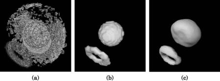
Figure 8.4 presents one slice from an MRI scan of a mouse embryo, and an isosurface model of its liver extracted from the unprocessed dataset. Figure 8.5 presents 3D renderings of the sequence of steps performed on the mouse MRI data to segment the liver. The first step is the initialization, which includes smoothing the input data, thresholding followed by a a flood fill to remove isolated holes, and finally applying morphological operators to remove small gaps and protrusions on the surface. The second (surface deformation) step