

Kluwer - Handbook of Biomedical Image Analysis Vol
.1.pdf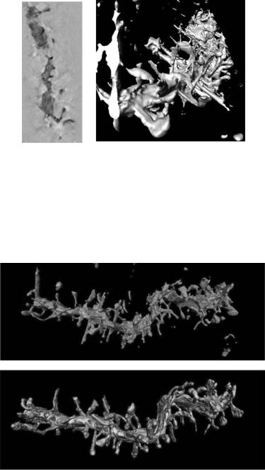
Level Set Segmentation of Biological Volume Datasets |
427 |
the “spines” that cover this dendrite. These types of “judgments” that humans make when they perform such tasks by hand are a mixed blessing. Humans can use high-level knowledge about the problem to fill in where the data is weak, but the expectations of a trained operator can interfere with seeing unexpected or unusual features in the data.
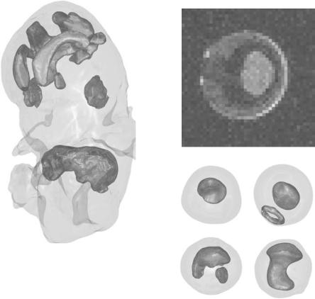
Figure 8.8(c) presents models from four samples of an MR series of a developing frog embryo. The top left image (hour 9) shows the first evident structure, the blastocoel, in blue, surrounded by the outside casing of the embryo in gray.
(b)
(a)
(c)
Figure 8.8: (a) Final mouse embryo model with skin (gray), liver (blue), brain ventricles (red), and eyes (green). (b) Hour 16 dataset. (c) Geometric structures extracted from MRI scans of a developing frog embryo, with blastocoel (blue), blastoporal lip (red), and archenteron (green). Hour 9 (top left), hour 16 (top right), hour 20 (bottom left), and hour 30 (bottom right).
428 |
|
|
|
Breen, Whitaker, Museth, and Zhukov |
Table 8.1: Parameters for processing example datasets |
||||
|
|
|
|
|
Dataset |
|
Initialization |
|
Surface Fitting |
|
|
|
|
|
Dendrite |
1. Gaussian blur σ = 0.5 |
1. |
Edge fitting: σ = 0.75, threshold = 6, β = 0.1 |
|
|
2. |
Threshold: I < 127 |
2. |
Gradient magnitude fitting: σ = 0.5, β = 1.0 |
|
3. |
Fill isolated holes |
|
|
|
4. |
Morphology: O0.5 ◦ C1.5 |
|
|
Mouse |
1. Gaussian blur σ = 0.5 |
1. |
Edge fitting: σ = 0.75, threshold = 20, β = 2 |
|
|
2. |
Threshold: I > 3, I < 60 |
2. |
Gradient magnitude fitting: σ = 0.5, β = 16.0 |
|
3. |
Fill isolated holes |
|
|
|
4. |
Morphology: O2.0 ◦ C3.0 |
|
|
Frog |
1. Interactive |
1. |
Gradient magnitude fitting: σ = 1.25, β = 1.0 |
|
The top right image (hour 16) demonstrates the expansion of the blastocoel and the development of the blastoporal lip in red. In the bottom left image (hour 20) the blastoporal lip has collapsed, the blastocoel has contracted, and the archenteron in green has developed. In the bottom right image (hour 30) the blastocoel has collapsed and only the archenteron is present. For this dataset it was difficult to isolate structures only based on their voxel values. We therefore used our interactive techniques to isolate (during initialization) most of the structures in the frog embryo samples.
Table 8.1 describes for each dataset the specific techniques and parameters we used for the results in this section. These parameters were obtained by first making a sensible guess based on the contrasts and sizes of features in the data and then using trial and error to obtain acceptable results. Each dataset was processed between four and eight times to achieve these results. More tuning could improve things further, and once these parameters are set, they work moderately well for similar modalities with similar subjects. The method is iterative, but the update times are proportional to the surface area. On an SGI 180 MHz MIPS 10000 machine, the smaller mouse MR dataset required approximately 10 min of CPU time, and the dendrite dataset ran for approximately 45 min. Most of this time was spent in the initialization (which requires several complete passes through the data) and in the edge detection. The frog embryo datasets needed only a few minutes of processing time, because they did not require computational initialization and are significantly smaller than the other example datatsets.
Level Set Segmentation of Biological Volume Datasets |
429 |
8.4Segmentation From Multiple Nonuniform Volume Datasets
Many of today’s volumetric datasets are generated by medical MR, CT, and other scanners. A typical 3D scan has a relatively high resolution in the scanning X– Y plane, but much lower resolution in the axial Z direction. The difference in resolution between the in-plane and out-of-plane samplings can easily range between a factor of 5 and 10, see Fig. 8.9. This occurs both because of physical constraints on the thickness of the tissue to be excited during scanning (MR), total tissue irradiation (CT), and scanning time restrictions. Even when time is not an issue, most scanners are by design incapable of sampling with high resolution in the out-of-plane direction, producing anisotropic “brick-like” voxels.
The nonuniform sampling of an object or a patient can create certain problems. The inadequate resolution in the Z direction implies that small or thin structures will not be properly sampled, making it difficult to capture them during surface reconstruction and object segmentation. One way to address this problem is to scan the same object from multiple directions, with the hope that the small structures will be adequately sampled in one of the scans. Generating several scans of the same object then raises the question of how to properly combine the information contained in these multiple datasets. Simply merging the individual scans does not necessarily assemble enough samples to produce a high resolution volumetric model. To address this problem we have developed a method for deforming a level set model using velocity information derived from multiple volume datasets with nonuniform resolution in order to produce a single high-resolution 3D model [43]. The method locally approximates the values of the multiple datasets by fitting a distance-weighted polynomial using moving least-squares (MLS) [44, 45]. Directional 3D edge information that may be used during the surface deformation stage is readily derived from MLS, and integrated within our segmentation framework.
The proposed method has several beneficial properties. Instead of merging all of the input volumes by global resampling (interpolation), we locally approximate the derivatives of the intensity values by MLS. This local versus global approach is feasible because the level set surface deformation only requires edge information in a narrow band around the surface. Consequently, the
430 |
Breen, Whitaker, Museth, and Zhukov |
MLS calculation is only performed in a small region of the volume, rather than throughout the whole volume, making the computational cost proportional to the object surface area [36]. As opposed to many interpolation schemes, the MLS method is stable with respect to noise and imperfect registrations [46]. Our implementation also allows for small intensity attenuation artifacts between the multiple scans thereby providing gain-correction. The distance-based weighting employed in our method ensures that the contributions from each scan are properly merged into the final result. If a slice of data from one scan is closer to a point of interest on the model, the information from this scan will contribute more heavily to determining the location of the point.
To the best of our knowledge there is no previous work on creating deformable models directly from multiple volume datasets. While there has been previous work on 3D level set segmentation and reconstruction [5, 6, 8, 41, 47], it has not been based on multiple volume datasets. However, 3D models have been generated from multiple range maps [29, 36, 48, 49], but the 2D nature of these approaches is significantly different from the 3D problem being addressed here. The most relevant related projects involve merging multiple volumes to produce a single high-resolution volume dataset [50,51], and extracting edge information from a single nonuniform volume [52]. Our work does not attempt to produce a high-resolution merging of the input data. Instead, our contribution stands apart from previous work because it deforms a model based on local edge information derived from multiple nonuniform volume datasets.
We have demonstrated the effectiveness of our approach on three multiscan datasets. The first two examples are derived from a single high-resolution volume dataset that has been subsampled in the X, Y, and Z directions. Since these nonuniform scans are extracted from a single dataset, they are therefore perfectly aligned. The first scan is derived from a high-resolution MR scan of a 12-day-old mouse embryo, which has already had its outer skin isolated with a previous segmentation process. The second example is generated from a laser scan reconstruction of a figurine. The third example consists of multiple MR scans of a zucchini that have been imperfectly aligned by hand. The first two examples show that our method is able to perform level set segmentation from multiple nonuniform scans of an object, picking up and merging features only found in one of the scans. The second example demonstrates that our method generates satisfactory results, even when there are misalignments in the registration.
Level Set Segmentation of Biological Volume Datasets |
431 |
8.4.1 Method Description
We have formulated our approach to 3D reconstruction of geometric models from multiple nonuniform volumetric datasets within our level set segmentation framework. Recall that speed function F() describes the velocity at each point on the evolving surface in the direction of the local surface normal. All of the information needed to deform a surface is encapsulated in the speed function, providing a simple, unified approach to evolving the surface. In this section we define speed functions that allow us to solve the multiple-data segmentation problem. The key to constructing suitable speed terms is 3D directional edge information derived from the multiple datasets. This problem is solved using a moving least-squares scheme that extracts edge information by locally fitting sample points to high-order polynomials.
8.4.1.1 Level Set Speed Function for Segmentation
Many different speed functions have been proposed over the years for segmentation of a single volume dataset [5, 6, 8, 41]. Typically such speed functions consist of a (3D) image-based feature attraction term and a smoothing term which serves as a regularization term that lowers the curvature and suppresses noise in the input data. From computer vision it is well known that features, i.e. significant changes in the intensity function, are conveniently described by an edge detector [53]. There exists a very large body of work devoted to the problem of designing optimal edge detectors for 2D images [14, 16], most of which are readily generalized to 3D. For this project we found it convenient to use speed functions with a 3D directional edge term that moves the level set toward the maximum of the gradient magnitude. This gives a term equivalent to Eq. (8.8),
Fgrad(x, n, φ) = αn · Vg , |
(8.10) |
where α is a scaling factor for the image-based feature attraction term Vg and n is the normal to the level set surface at x. Vg symbolizes some global uniform merging of the multiple nonuniform input volumes. This feature term is effectively a 3D directional edge detector of Vg . However, there are two problems associated with using this speed function exclusively. The first is that we cannot expect to compute reliable 3D directional edge information in all regions of space simply because of the nature of the nonuniform input volumes. In

432 |
Breen, Whitaker, Museth, and Zhukov |
other words, Vg cannot be interpolated reliably in regions of space where there are no nearby sample points. Hence the level set surface will not experience any image-based forces in these regions. The solution is to use a regularization term that imposes constraints on the mean curvature of the deforming level set surface. We include the smoothing term from Eq. (8.6) and scale it with parameter β, in order to smooth the regions where no edge information exists as well as suppress noise in the remaining regions, thereby preventing excessive aliasing.
Normally the feature attraction term, Vg , creates only a narrow range of influence. In other words, this feature attraction term will only reliably move the portion of the level set surface that is in close proximity to the actual edges in Vg . Thus, a good initialization of the level set surface is needed before solving the level set equation when using Fgrad (Eq. (8.10)). A reasonable initialization of the level set surface may be obtained by computing the CSG union of the multiple input volumes, which are first trilinearly resampled to give a uniform sampling. However, if the input volumes are strongly nonuniform, i.e. they are severely undersampled in one or more directions, their union produces a poor initial model. To improve the initialization we attract the CSG union surface to the Canny edges [16] computed from Vg using the distance transform produced from those edges (see Eq. (8.7)). This approach allows us to move the initial surface from a long range, but only with pixel-level accuracy.
Canny edges are nondirectional edges defined from the zero-crossing of the second derivative of the image in the direction of the local normal. In 3D this is
∂2 |
|
∂n2g Vg = 0, |
(8.11) |
where ng ≡ Vg / Vg is the local normal vector of Vg . Using the expression
∂/∂ng = ng · , we can rewrite Eq. (8.11) as
∂2 |
ng · Vg = ng · Vg . |
|
∂n2g Vg = ng · |
(8.12) |
The next section focuses on the methods needed to reliably compute the vectors ng and Vg . In preparation, the latter may be explicitly expressed in terms of the derivatives of the merged volume Vg ,
|
|
|
|
|
|
|
V |
Vg |
HVg |
, |
(8.13) |
g = |
|
Vg |
|
||
