

Kluwer - Handbook of Biomedical Image Analysis Vol
.1.pdfWavelets in Medical Image Processing |
|
315 |
wavelet ψ (x) = g(t)eiηt is then obtained with a Gaussian function |
||
|
1 |
−t2 |
g(t) = |
|
e 2σ 2 |
(σ 2π )1/4 |
||
(see [14]).
Extension of Gabor wavelet to 2D is expressed as:
ψ k(s, y) |
= |
g(x, y)e−iη(x cos αk)+y sin αk). |
(6.24) |
|
|
|
Different translation and scaling parameters of ψ k(x, y) constitute the wavelet basis for expansion. An extra parameter αk provides selectivity for the orientation of the function. We observe here that the 2D Gabor wavelet has a nonseparable structure that provides more flexibility on orientation selection than separable wavelet functions.
It is well known that optical sensitive cells in animal’s visual cortex respond selectively to stimuli with particular frequency and orientation [26]. Equation (6.24) described a wavelet representation that naturally reflects this neurophysiological phenomenon. Gabor expansion and Gabor wavelets have therefore been widely used for visual discrimination tasks and especially texture recognition [27, 28].
6.2.3.2 Wavelet Packets
Unlike dyadic wavelet transform, wavelet packets decompose the low-frequency component as well as the high-frequency component in every subbands [29]. Such adaptive expansion can be represented with binary trees where each subband highor low-frequency component is a node with two children corresponding to the pair of highand low-frequency expansion at the next scale. An admissible tree for an adaptive expansion is therefore defined as a binary tree where each node has either 0 or 2 children, as illustrated in Fig. 6.6(c). The number of all different wavelet packet orthogonal basis (also called a wavelet packets dictionary) is equal to the number of different admissible binary trees, which is of the order of 22J , where J is the depth of decomposition [14].
Obviously, wavelet packets provide more flexibility on partitioning the spatial-frequency domain, and therefore improve the separation of noise and signal into different subbands in an approximated sense (this is referred to the near-diagonalization of signal and noise). This property can greatly facilitate

316 |
Jin, Angelini, and Laine |
Figure 6.6: (a) Dyadic wavelet decomposition tree. (b) Wavelet packets decomposition tree. (c) An example of an orthogonal basis tree with wavelet packets decomposition.
the enhancement and denoising task of a noisy signal if the wavelet packets basis are selected properly [30]. In practical applications for various medical imaging modalities and applications, features of interest and noise properties have significantly different characteristics that can be efficiently characterized separately with this framework.
A fast algorithm for wavelet-packets best basis selection was introduced by Coifman and Wickerhauser in [30]. This algorithm identifies the “best” basis for a specific problem inside the wavelet packets dictionary according to a criterion (referred to as a cost function) that is minimized. This cost function typically reflects the entropy of the coefficients or the energy of the coefficients inside each subband and the optimal choice minimizes the cost function comparing values at a node and its children. The complexity of the algorithm is O (N log N) for a signal of N samples.
6.2.3.3 Brushlets
Brushlet functions were introduced to build an orthogonal basis of transient functions with good time–frequency localization. For this purpose, lapped orthogonal transforms with windowed complex exponential functions, such as Gabor functions, have been used for many years in the context of sine–cosine transforms [31].
Brushlet functions are defined with true complex exponential functions on subintervals of the real axis as:
uj,n(x) = bn(x − cn)e j,n(x) + v(x − an)e j,n(2an − x)−v(x − an+1)e j,n(2an+1 −x),
(6.25)

Wavelets in Medical Image Processing |
317 |
where ln = an+1 − an and cn = ln/2. The two window functions bn and v are
derived from the ramp function r:
0 if t ≤ −1
r(t) = (6.26)
1if t ≥ 1
and
r2(t) + r2(−t) = 1, t R. |
(6.27) |
The bump function v is defined as:
|
v(t) = r |
t |
|
|
|
ε |
|||
The bell function bn is defined by: |
|
|||
|
l |
2 |
if |
|
|
r2 t +εn/ |
|
||
|
|
|
|
|
|
ε |
|
|
|
|
r |
−t |
, t |
|
[ε, ε]. |
(6.28) |
|
|
t [−ln/2 − ε, −ln/2 + ε]
bn(t) = 1 |
|
|
− t |
if t [−ln/2 + ε, ln/2 − ε]. |
(6.29) |
||||
r2 |
ln/ |
2 |
if t [ln/2 − ε, ln/2 + ε] |
|
|||||
ε |
|
||||||||
|
|
|
|
|
|
|
|
|
|
|
|
|
|
|
|
|
|
|
|
|
|
|
|
|
|
|
|
|
|
An illustration of the windowing functions is provided in Fig. 6.7. |
|
||||||||
|
|
|
|
|
|
|
|
|
|
Finally, the complex-valued exponentials e j,n are defined as: |
|
||||||||
|
|
|
|
1 |
|
2iπ j (x−an) |
(6.30) |
||
|
|
|
e j,n(x) = |
√ |
|
e− |
ln . |
||
|
|
|
|
|
ln |
|
|
||
In order to decompose a given signal f along directional texture components, the Fourier transform fˆ of the signal and not the signal itself is projected on the
2 e |
|
|
ln |
|
2 e |
1 |
|
|
|
|
|
0.5 |
|
|
bn ( x ) |
|
|
|
|
|
|
|
|
|
v ( x ) |
|
|
|
|
an − e |
an |
an + e |
an + 1 − e |
an + 1 |
an + 1 |
|
|
|
|
v ( x ) |
|
Figure 6.7: Windowing functions bn and bump functions ν defined on the interval [an − ε, an+1 + ε].

318 |
Jin, Angelini, and Laine |
brushlet basis functions: |
|
fˆ = fˆn, j un, j , |
(6.31) |
nj
with un, j being the brushlet basis functions and fˆn, j |
being the brushlet coeffi- |
cients. |
|
The original signal f can then be reconstructed by: |
|
f = fˆn, j wn, j , |
(6.32) |
nj
is the inverse Fourier transform of un, j , which is expressed as:
|
( |
) |
|
l |
|
e |
2iπ anx |
e |
iπlnx |
( |
|
1) |
j ˆ |
(l |
|
x |
|
j) |
|
2i sin(πl |
|
x)vˆ (l |
|
x |
|
j) , |
wn, j |
|
x |
= |
|
n |
|
|
|
|
) |
− |
|
bn |
|
n |
|
− |
|
− |
|
n |
|
n |
|
+ |
*(6.33) |
ˆ
with bn and vˆ being the Fourier transforms of the window functions bn and v. Since the Fourier operator is a unitary operator, the family of functions wn, j is also an orthogonal basis of the real axis. We observe here the wavelet-like structure of the wn, j functions with scaling factor ln and translation factor j. An illustration of the brushlet analysis and synthesis functions is provided in Fig. 6.8.
Projection on the analysis functions un, j can be implemented efficiently by a folding operator and Fourier transform. The folding technique was introduced by Malvar [31] and is described for multidimensional implementation by Wickerhauser in [21]. These brushlet functions share many common properties with Gabor wavelets and wavelet packets regarding the orientation and frequency selection of the analysis but only brushlet can offer an orthogonal framework
10−1 |
|
|
10−2 |
|
2 |
|
5 |
|
|
0 |
|
0 |
|
|
−2 |
time |
−5 |
|
frequency |
|
- j |
|
||
an - e |
an+1 + e |
|
j |
|
|
|
|
ln |
ln |
|
(a) |
|
|
(b) |
Figure 6.8: (a) Real part of analysis brushlet function un, j . (b) Real part of |
||||
synthesis brushlet function wn, j . |
|
|
|
|
Wavelets in Medical Image Processing |
319 |
with a single expansion coefficient for a particular pair of frequency and orientation.
6.3Noise Reduction and Image Enhancement Using Wavelet Transforms
Denoising can be viewed as an estimation problem trying to recover a true signal component X from an observation Y where the signal component has been degraded by a noise component N:
Y = X + N. |
(6.34) |
The estimation is computed with a thresholding estimator in an orthonormal basis B = {gm}0≤m<N as [32]:
ˆ |
N−1 |
|
X = |
|
|
ρm( X, gm )gm, |
(6.35) |
m=0
where ρm is a thresholding function that aims at eliminating noise components (via attenuating or decreasing some coefficient sets) in the transform domain while preserving the true signal coefficients. If the function ρm is modified to rather preserve or increase coefficient values in the transform domain, it is possible to enhance some features of interest in the true signal component with the framework of Eq. (6.35).
Figure 6.9 illustrates a multiscale enhancement and denoising framework using wavelet transforms. An overcomplete dyadic wavelet transform using biorthogonal basis is used. Notice that since the DC cap contains the overall energy distribution, it is usually not thresholded during the procedure. As shown in this figure, thresholding and enhancement functions can be implemented independently from the wavelet filters and easily incorporated into the filter bank framework.
6.3.1 Thresholding Operators for Denoising
As a general rule, wavelet coefficients with larger magnitude are correlated with salient features in the image data. In that context, denoising can be achieved by applying a thresholding operator to the wavelet coefficients (in the transform

320 |
Jin, Angelini, and Laine |
T1
T2
Wavelet |
|
|
|
Wavelet |
Decomposition |
|
T3 |
|
Reconstruction |
|
|
|
|
Input Image
Output Image
DC
Figure 6.9: A Multiscale framework of denoising and enhancement using discrete dyadic wavelet transform. A three-level decomposition was shown.
domain) followed by reconstruction of the signal to the original image (spatial) domain.
Typical threshold operators for denoising include hard thresholding:
|
|
ρT (x) = |
|
x, |
if |
|x| > T , |
|
|
(6.36) |
||||||||||
|
|
|
|
|
|
|
|
|
0, |
if |
|x| ≤ T |
|
|
|
|
||||
soft thresholding (wavelet shrinkage) [33]: |
|
|
|
|
|
|
|
|
|||||||||||
|
|
|
|
|
= |
|
x |
+ |
T, |
if |
x |
≤ − |
|
|
|
||||
|
|
|
|
|
|
|
|
|
− T, |
|
x ≥ |
|
|
|
|
|
|||
|
ρT (x) |
|
|
x |
if |
|
|
T, |
|
(6.37) |
|||||||||
|
|
|
|
|
|
|
|
0, |
|
if |
|x| < T |
|
|
||||||
and affine (firm) thresholding |
[34]: |
|
|
|
|
|
|
|
|
|
|
|
|||||||
|
|
|
|
|
|
|
|
|
|
|
|
|
|
||||||
|
|
|
|
x, |
|
|
|
|
if |
x ≥ T |
|
|
|
|
|
|
|||
|
|
|
|
|
|
|
|
|
|
| | T |
|
|
|
|
|
|
|
|
|
|
|
|
|
|
|
|
− |
|
|
|
≤ |
|
|
≤ |
|
|
|||
|
|
|
|
2x |
T, |
if |
|
|
T/2 |
|
|||||||||
ρT (x) |
|
|
+ |
≤ |
x |
≤ − |
(6.38) |
||||||||||||
= |
|
|
|
|
|
|
|
− |
|
|
. |
||||||||
|
|
|
2x T, if T/2 |
|
x T |
|
|
||||||||||||
|
|
|
|
|
|
|
|
|
|
|
|
|
|
|
|
|
|
|
|
|
|
|
|
|
|
|
|
|
|
|
|
|
|
|
|
|
|
|
|
|
|
|
|
0, |
|
|
|
|
if |
|x| < T |
|
|
|
|
|
|
|||
|
|
|
|
|
|
|
|
|
|
|
|
|
|
||||||
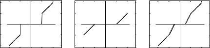
The shapes of these |
thresholding operators are illustrated in Fig. 6.10. |
|
|||||||||||||||||
|
|
|
|
|
|
|
|
|
|
|
|
|
|
|
|
|
|
|
|
6.3.2 Enhancement Operators
Magnitude of wavelet coefficients measures the correlation between the image data and the wavelet functions. For first-derivative-based wavelet, the magnitude
Wavelets in Medical Image Processing
1 |
|
|
|
|
0.5 |
|
|
|
|
0 |
|
|
|
|
−0.5 |
|
|
|
|
−1 |
|
|
|
|
−1 |
−0.5 |
0 |
0.5 |
1 |
|
|
(a) |
|
|
1 |
1 |
0.5 |
0.5 |
0 |
0 |
−0.5 |
−0.5 |
−1 |
−1 |
−1 −0.5 0 |
0.5 1 |
(b)
|
|
|
|
321 |
−1 |
−0.5 |
0 |
0.5 |
1 |
|
|
(c) |
|
|
Figure 6.10: Example of thresholding functions, assuming that the input data was normalized to the range of [−1, 1]. (a) Hard thresholding, (b) soft thresholding, and (c) affine thresholding. The threshold level was set to T = 0.5.
therefore reflects the “strength” of signal variation. For second-derivative-based wavelets, the magnitude is related to the local contrast around a signal variation. In both cases, large wavelet coefficient magnitude occurs around strong edges. To enhance weak edges or subtle objects buried in the background, an enhancement function should be designed such that wavelet coefficients within certain magnitude range are amplified.
General guidelines for designing a nonlinear enhancement function E(x) are [35]:
1.An area of low contrast should be enhanced more than an area of high contrast. This is equivalent to saying that smaller values of wavelet coefficients should be assigned larger gains.
2.A sharp edge should not be blurred.
In addition, an enhancement function may be further subjected to the following
constraints [36]:
1.Monotonically increasing: Monoticity ensures the preservation of the relative strength of signal variations and avoids changing location of local extrema or creating new extrema.
2.Antisymmetry: (E(−x) = −E(x)): This property preserves the phase polarity for “edge crispening.”
A simple piecewise linear function [37] that satisfies these conditions is plotted in Fig. 6.11(a):
|
= |
|
x (K − 1)T, |
| | ≤ |
|
|
|
|
|
|
− K x, |
|
|
E(x) |
|
|
|
if x T. |
(6.39) |
|
|
|
|
|
+ (K − 1)T, |
if x > T |
|
|
|
x |
|
|||

322 |
Jin, Angelini, and Laine |
5 |
|
|
|
|
|
1 |
|
|
|
|
4 |
|
|
|
|
|
|
|
|
|
|
|
|
|
|
|
|
|
|
|
|
|
3 |
|
|
|
|
|
|
|
|
|
|
2 |
|
|
|
|
|
0.5 |
|
|
|
|
|
|
|
|
|
|
|
|
|
|
|
1 |
|
|
|
|
|
|
|
|
|
|
0 |
|
|
|
|
|
0 |
|
|
|
|
−1 |
|
|
|
|
|
|
|
|
|
|
−2 |
|
|
|
|
|
−0.5 |
|
|
|
|
−3 |
|
|
|
|
|
|
|
|
|
|
|
|
|
|
|
|
|
|
|
|
|
−4 |
|
|
|
|
|
−1 |
|
|
|
|
−5 |
|
|
|
|
|
|
|
|
|
|
−1 |
−0.5 |
0 |
0.5 |
1 |
−1 |
−0.5 |
0 |
0.5 |
1 |
|
|
|
|
(a) |
|
|
|
|
(b) |
|
|
Figure 6.11: Example of enhancement functions, assuming that the input data was normalized to the range of [−1, 1]. (a) Piecewise linear function, T = 0.2,
K = 20. (b) Sigmoid enhancement function, b = 0.35, c = 20. Notice the different scales of the y-axis for the two plots.
Such enhancement is simple to implement, and was used successfully for contrast enhancement on mammograms [19, 38, 39].
From the analysis in the previous subsection, wavelet coefficients with smallmagnitude were also related to noise. A simple amplification of small-magnitude coefficients as performed in Eq. (6.39) will certainly also amplify noise components. This enhancement operator is therefore limited to contrast enhancement of data with very low noise level, such as mammograms or CT images. Such a problem can be alleviated by combining the enhancement with a denoising operator presented in the previous subsection [35].
A more careful design can provide more reliable enhancement procedures with a control of noise suppression. For example, a sigmoid function [37], plotted in Fig. 6.11 (b), can be used:
E(x) = a[sigm(c(x − b)) − sigm(−c(x + b))], |
(6.40) |
|||||||||||
where |
|
|
|
|
|
|
|
|
|
|
|
|
|
|
|
|
1 |
|
|
|
|
|
0 < b < 1, |
|
|
|
|
|
|
|
|
|
|
|
|
|
|
|
a = sigm(c(1 |
− |
b)) |
− |
sigm( |
− |
c(1 |
+ |
b)) |
, |
|
||
|
|
|
|
|
||||||||
1
and sigm(y) is defined as sigm(y) = 1 + e−y . The parameters b and c respectively control the threshold and rate of enhancement. It can be easily shown that E(x) in Eq. (6.40) is continuous and monotonically increasing within the interval

Wavelets in Medical Image Processing |
323 |
[−1, 1]. Furthermore, any order of derivatives of E(x) exists and is continuous. This property avoids creating any new discontinuities after enhancement.
6.3.3 Selection of Threshold Value
Given the basic framework of denoising using wavelet thresholding as discussed in the previous sections, it is clear that the threshold level parameter T plays an essential role. Values too small cannot effectively get rid of noise component, while values too large will eliminate useful signal components. There are a variety of ways to determine the threshold value T as will be discussed in this section.
Depending on whether or not the threshold value T changes across wavelet scales and spatial locations, the thresholding can be:
1.global threshold: a single value T is to be applied globally to all empirical wavelet coefficients at different scales. T = const.
2.level-dependent threshold: a different threshold value T is selected for each wavelet analysis level (scale). T = T( j), j = 1, . . . , J, J being the coarsest level for wavelet expansion to be processed.
3.spatial adaptive threshold: the threshold value T varies spatially depending on local properties of individual wavelet coefficients. Usually, T is also level dependent. T = Tj (x, y, z).
While a simple way of determining T is as a percentage of coefficients maxima, there are different adaptive ways of assigning the T value according to the noise level (estimated via its variance σ ):
√
1.universal threshold: T = σ 2 log n [40], with n equal to the sample size. This threshold was determined in an optimal context for soft thresholding with random Gaussian noise. This scheme is very easy to implement, but typically provides a threshold level larger than with other decision criteria, therefore resulting in smoother reconstructed data. Also such estimation does not take into account the content of the data, but only depends on the data size.
2.minimax threshold: T = σ Tn [41], where Tn is determined by a minimax rule such that the maximum risk of estimation error across all locations of
324 |
Jin, Angelini, and Laine |
the data is minimized. This threshold level depends on the noise and signal relationships in the input data.
3.stein unbiased estimated of risk: Similar to minimax threshold but Tn is determined by a different risk rule [42, 43].
4.spatial adaptive threshold: T = σ 2/σX [44], where σX is the local variance of the observation signal, which can be estimated using a local window moving across the image data or, more accurately, by a context-based clustering algorithm.
In many automatic denoising methods to determine the threshold value T, an estimation of the noise variance σ is needed. Donoho et al. [45] proposed a robust estimation of noise level σ based on the median absolute value of the wavelet coefficients as:
σ = |
median(|W1(x, y, z)|) |
, |
(6.41) |
|
|||
0.6745 |
|
|
|
where W1 is the most detailed level of wavelet coefficients. Such estimator has become very popular in practice and is widely used.
6.3.4 Summary
In general, multiscale denoising techniques involve a transformation process and a thresholding operator in the transform domain. Research dedicated to the improvement of such a technique has been explored along both directions. Various multiscale expansions have been proposed, aimed at better adaptation to signal and feature characteristics. Traditionally, an orthogonal base was used for expansion [33], which leads to a spatial-variant transform. Various artifacts, e.g. pseudo-Gibbs phenomena, were exhibited in the vicinity of discontinuities. Coifman et al. [40] proposed a translation-invariant thresholding scheme, which averages several denoising results on different spatial shifts of the input image. Laine et al. [38] prompted to an overcomplete representation which allows redundancy in the transform coefficients domain and provides a translation-invariant decomposition. Wavelet coefficients in an overcomplete representation have the same size as the input image, when treated as a subband image. Many denoising and enhancement techniques can be applied within a