Kluwer - Handbook of Biomedical Image Analysis Vol

E = F(x, y, Z, p, q)dx dy.

E has an extremum only if the Euler differential equation

is satisfied. If the solution is subject to the constraints g j (x, y, Z) = 0, j = 1, . . . , k,

then we have

k

G = F + λ j g j (x, y, Z).

j=1

Now the Euler equation is

The λ j ’s are called Lagrange multipliers. An example is provided in Section

5.3.2.1.

5.2.3.2 The Constraint Functions Used in SFS Models

When iterative algorithms are used for solving the SFS problem, constraints will be proposed to secure a weak solution. The following constraints are examples:

(1) total squared brightness error [27]:

G0 = (I(x, y) − R( p, q))2dx dy. (5.14)

(2) weak smoothness: After the tangent planes are available, the surface Z

is reconstructed by minimizing the following functional:

G1 = ( px2 + p2y + qx2 + qy2)dx dy. (5.15)

(3)integrability: Since p and q are considered independent variables, ( p, q) may not correspond to the orientation of the underlying surface Z, that is, the surface Z cannot be derived by integrating Zx = p, Zy = q. An

derivatives are discretized by using “difference” and (2) solving the derived difference equation—an algebraic equation—by using either an iterative or a direct method.

To begin with, we first partition the domain by a mesh grid. For example, we use a uniform mesh grid with grid lines:

where h = xi+1 − xi and k = yi+1 − yi are the mesh sizes in the x and ydirections, respectively. For simplicity, we write fj,l = f (xj , yl ), the function values on the nodes of the mesh.

Using Taylor expansion and intermediate value theorem, we can derive the following numerical differentiation formulas:

forward difference formula:

Formulas (5.23–5.26) will be used in Section 5.3 to discretize (or linearize) the irradiance equation (5.2).

We now demonstrate the idea of FDM by the following examples.

Example 3. As an example, we consider using FDM to solve the linear shape from shading problem (5.3) on a square domain:

= {(x, y), 0 < x < 1, 0 < y < 1}

with the boundary condition given by (5.4). Using forward difference formula (5.23), we have

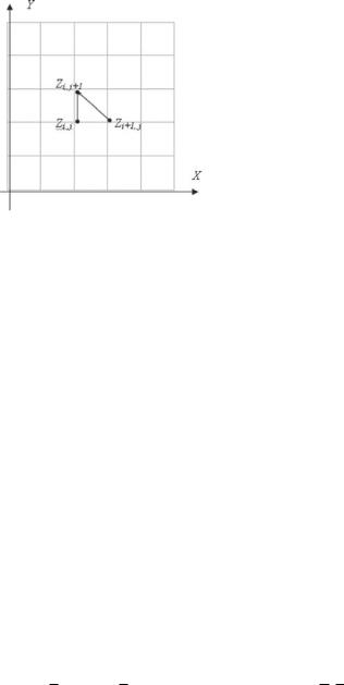
Figure 5.1 shows the discretization we are using.

The finite difference scheme (5.29) is called the explicit method since it is given by an iterative formula. If instead, the central (5.25) and forward difference formulas (5.23) are used to approximate the partial derivatives, an implicit finite difference scheme can be derived. The approximate solution is then derived iteratively by using the iteration formula (5.29). Numerical

Figure 5.1: The grid mesh for the discretization in Example 3.

methods used to solve these matrix equations, for example, the Jacobi method, can be found in the standard numerical analysis textbooks [24].

For a nonlinear shape from shading model (5.5), we have to linearize the reflectance map by using Taylor expansion to get a linear equation and then apply the FDM in a similar way as in the above example. To linearize the equation, we only need to replace the nonlinear part in Eq. (5.2) by its linear approximation. We first rewrite the equation to separate the linear and nonlinear parts:

where the error term O (|( p − p)2 + (q − q)2|) depends on the value of ( p, q)

and the smoothness of the solution function Z. If we assume that Z C2( ), then this error term can be ignored locally. Now we substitute (5.30) into (5.31) to have the linearized irradiance equation:

where

P(x, y) = − pI(x, y) + ρp0,

Q(x, y) = −q I(x, y) + ρq0,

Note that (5.32) is a first-order partial differential equation with nonconstant coefficients P and Q and, therefore, the FDM can be used to solve it in the same way as in Example 2.

5.2.4.2 Remarks

Remark 2. About convergence of finite difference method. Every numerical method provides a formalism of generating discrete algorithms for approximating the solution of a PDE. Such a task could be done automatically by a computer if there were no mathematical skills that require human involvement. Consequently, it is necessary to understand the mathematics in this black box which you put in your PDE for processing. This will involve discussion on convergence, stability, and error analysis. However, these topics are beyond the scope of this introductory chapter. We hope the loose ends left here will stimulate your curiosity and further motivate your deep interest in this subject. For the finite difference method used to solve the SFS model, some results related to the issue of convergence can be found in Ulich [64]. For the linear problem, Ulich proved convergence for three methods: forward difference method, backward difference method, and central and forward difference method for certain light directions. For the central and forward finite difference method applied to the linear PDE derived from linearization of a nonlinear shape from shading problem, she was able to prove convergence for all light directions. For the case of application of FDM to the linear shape from shading models, Wei et al. [65] discussed the convergence properties for four explicit, two implicit, and four semi-implicit finite difference algorithms. They also give comparisons of accuracy, solvability, stability, and convergence of these schemes.

Remark 3. About Multiscale methods. Simple iterative methods (such as the Jacobi method) tend to damp out high-frequency components of the error faster than any other method. Multiscale methods are introduced to

improve the convergence and accuracy of the numerical solutions derived in the “single scale” methods. The multigrid method appears to be one of the most successful multiscale methods for solving the SFS problems. The multigrid method associated with vision problems was studied in the early 1960s by Fedorenko and Bakhvalov [3] and later in the work of many others, for example, [1, 56, 57]. For readers without previous experiences in the multigrid method, excellent tutorials can be found in the books [8] and [44, 62]. A classic book on multigrid method is [23]. Some other novel multiscale methods are developed recently, for example, the panel-clustering method, waveletbased matrix compression, and the hierarchical matrix decomposition technique.

5.3Numerical Algorithms and Their Implementations

It is understood that the problem of shape from shading is fundamentally a very difficult mathematical problem. Nevertheless, some methods were developed while attempting to solve the problem numerically for some particular cases. Most of the methods work for a particular type of images.

SFS techniques can be roughly divided into four groups:

(1)Minimization approach. The method is to reconstruct the shape of the object by minimizing the well-designed energy function over the entire image. The idea is similar to that in deformable models used in image segmentation which segment the object by minimizing certain predefined energy functions. The constraint functions can be the brightness constraint, the gradient constraint, the smooth constraint, etc. (See Section 5.2.3.2).

(2)Propagation approach. The method starts from some initial curve, which is defined as special points such as the brightest or the darkest points in the image, and propagates the shape information across the entire image. (See 5.2.2).

(3)Local approach. The method reconstructs the shape by assuming local surface type. The surface is derived by matching derivatives of measured intensity to those assumed spherical surface.

Denoting by τ the tilt of the illuminant and by γ the slant of the illuminant, the above equation can be rewritten as

Using forward difference formula (5.23), we have

By taking Fourier transform on the two sides of Eq. (5.36), we can get the following results:

Substituting Eq. (5.37) into Eq. (5.35) and taking Fourier transform on both sides, we obtain

FI (w1, w2) = FZ (w1, w2)(−iw1) cos τ sin σ + FZ (w1, w2)(−iw2) sin τ sin σ,

(5.38) where FI (w1, w2) and FZ (w1, w2) are the Fourier transform of the input image

I(x, y) and depth map Z(x, y), respectively.

After rearranging Eq. (5.38), we obtain

It is obvious that this approach does not need iterative computation and can provide an approximate solution quickly. However, like all the other linear approaches, this method makes an assumption that the reflectance map is locally linear. Comparing Eq. (5.35) with the normal reflectance equation: