Kluwer - Handbook of Biomedical Image Analysis Vol

We observe that the linear method ignores the quadratic terms in Eq. (5.41). If we have a 3D object which has rapid changes in depth, both p and q will dominate

R( p, q), Pentland’s algorithm may not provide promising results. Fortunately, some objects do change smoothly so that linear approximation is satisfactory to certain extent.

The algorithm can be described by the following procedure:

Step 1. Input the original parameters of the reflectance map,

Step 2. Calculate the Fourier transform of the depth map Z(w1, w2) using Eq. (5.39),

Step 3. Calculate the inverse Fourier transform of the depth map Z(x, y) using Eq. (5.40).

The way to realize Pentland’s algorithm can be described by the following

pseudocode.

Algorithm 1. Pentland’s algorithm

Input Zmin (mindepthvalue), Zmax (maxdepthvalue), (x, y, z)(direction of the

end do

end do

Normalize(Z(x, y), Zmax , Zmin) Output Z(x, y)

The subfunctions FFT, IFFT, and Normalize are all standard math functions used in signal and image processing.

We now demonstrate this method by using the following example.

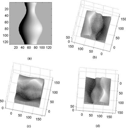
Example 4. Reconstruct the surface of a synthetic vase using Pentland’s method. The experiments are based on the synthetic images that are generated using true depth maps. Figure 5.2(a) shows the synthetic vase and the reconstruction results using Pentland’s algorithm. The light is from above at (x = 1,

this method discretizes the reflectance map in a different way. Like Pentland’s method, the surface orientation ( p, q) is approximated by its linear approximation using the forward difference formula (5.36), while unlike Pentland’s method, the reflectance map is then directly linearized in terms of the depth Z using Taylor series expansion. Finally, Newton’s iteration method is applied to the discretized equation to get a numerical approximation to the depth Z. In what follows, we will derive this scheme step by step.

To begin with, we rewrite the irradiance equation (5.2) in the following format:

Replacing p and q by their linear approximation using the forward difference formulas (5.36), we obtain

0 = f (I(x, y), Z(x, y), Z(x − 1, y), Z(x, y − 1))

= I(x, y) − R(Z(x, y) − Z(x − 1, y), Z(x, y) − Z(x, y − 1)). (5.43)

If we take the Taylor series expansion about a given depth map Zn−1, we get the following equation:

0= f (I(x, y), Z(x, y), Z(x − 1, y), Z(x, y − 1))

≈f (I(x, y), Zn−1(x, y), Zn−1(x − 1, y), Zn−1(x, y − 1))

+(Z(x, y) − Zn−1(x, y))

each value of the depth map can be iteratively calculated. In fact, (5.44) can be read as

By iteratively using formula (5.46), we obtain the approximation of the depth map Z(x, y). Readers may have noticed that the iterative formula is Newton’s formula.

This method has a similar disadvantage as the algorithm based on linear approach. However, it is faster since it does not need to compute the FFT and IFFT.

The algorithm can be described by the following procedure:

Step 1. Input the original parameters of the reflectance map,

Step 2. Set the initial guess of Z0(x, y) = 0,

Step 3. Refine the depth map Zk(x, y) using Eq. (5.46).

The way to realize Pentland’s algorithm can be described by the following pseudocode.

Algorithm 2: Tsai–Shah’s linearization method

Input Zmin(mindepthvalue), Zmax(maxdepthvalue), (x, y, z)(direction of the light source), I(x, y)(inputimage)

z0 ← 0;

p0 ← q0 ← 0;

p ← q ← p0 ← q0;

D ← x2 + y2 + z2, sx ← x/D, sy ← y/D, sz ← z/D. sin γ ← sin(arccos (lz)), sin τ ← sin(arctan(sy/sx)), cos τ ← cos(arctan (sy/sx)).

p ← Z(i, j) − Z(i, j − 1) q ← Z(i, j) − Z(i − 1, j)

end do

end do

Normalize(Z(x, y), Zmax, Zmin) O utput Z(x, y)

The subfunction Normalize is a standard math function used in signal and image processing.

We now demonstrate this method by using the following example.

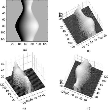
Example 5. Reconstruct the surface of a synthetic vase using Tsai–Shah’s method.

In order to compare with Pentland’s method, here we consider reconstruction of the same surface as in Example 2—the surface of a synthetic vase. Figure 5.3 shows the synthetic vase and the reconstruction results using Tsai– Shah’s algorithm from three different directions. The light is from above at (x = 0, y = 0, z = 1). The input image is showed in Fig. 5.3(a). The surface, shown in Fig. 5.3(b), (c), and (d), is the reconstructed surface from three different directions. Tsai–Shah’s algorithm works well and produces good results as expected for the vase. However, it is sensitive to noises as we will point out in the next section. In general, the experiment shows that Tsai–Shah’s algorithm can reconstruct the object well on the surface where the reflectance changes linearly with respect to the surface shape.

5.3.2 Optimization Approaches

As we pointed out earlier, the problem of recovering the shape from shading can be based on solving the irradiance equation (5.2). The irradiance equation is a first-order PDE. Unfortunately, in general, this PDE is nonlinear and only well posed under limited conditions. To make things worse, in practice,

Figure 5.3: Tsai–Shah’s linear SFS algorithm applied to the synthetic vase image. (a) is the input image with light source (x = 1, y = 0, z = 1). (b), (c), and

(d) are the reconstructed surface from three different directions.

the data available for shape reconstruction is not the complete intensity function, but rather its sampled version—a discrete data set. In addition, the reflectance map is usually determined experimentally as well. Usually people believe that the problem has at least one solution, but it is clear that the uniqueness of the solution is difficult to get. The optimization approach is one of the earliest approaches that has been proposed and researched for several decades. The original work can be traced back to the Ph.D. thesis of Horn [26]. Different constraint functions (see Section 5.2.3.2) can be used to minimize the energy function. First, we consider a general way to construct

the energy function, which contains almost all the common constraints listed in Section 5.2.3.2,

+ ((Zx − p)2 + (Zy − q)2) + ((Rx − Ix)2 + (Ry − Iy)2)}dx dy, (5.48)

−→

where N is defined as the surface normal, I is the input image, R is the reflectance map, (x, y) is an arbitrary pixel of the input image, and ( p, q) is orientation at pixel (x, y). The first term, (I − R)2, is called the brightness error term, which is used to minimize the brightness error between the measured image intensity and the reflectance function. The second tern, ( px2 + p2y + qx2 + qy2), is called the regularization term which will always penalize large local changes in

the surface orientation and encourage the surface change gradually. The third

||−→||2 −

term, ( N 1), is called unit normal term and is used to normalize the constraints on the recovered normal by forcing the surface normal to be unit vectors. The fourth term, ((Zx − p)2 + (Zy − q)2), is called integrability term which is used to ensure the valid surface. The last term, (Rx − Ix)2 + (Ry − Iy)2, is defined as the intensity gradient term. It requires that the intensity gradient of the reconstructed image be close to the intensity gradient of the input image in the x and y directions as much as possible. Sometimes, if an algorithm is designed for a particular type of images, adequate constraints should be chosen to meet some specific requirements.

In the following context we will introduce the most popular algorithm which is based on the concept of optimization.

5.3.2.1 Zheng and Chellappa’s minimization method

Zheng–Chellappa [70] chose the squared brightness error term (5.14), the integrability term, and the intensity gradient term as their energy function, which is defined to be

Recall that most of the traditional methods enforce the requirement that the reconstructed (approximated) image should be close to the input (exact) image,

where p = ∂ Z/∂ x and q = ∂ Z/∂ y, Z(x, y) is the height of image at (x, y).

Notice that, for each pixel, the right side of Eq. (5.2) is given values and in the left side p and q are free variables. Therefore, we write p = p(x, y) and

Using the technique of calculus of variations in Section 5.2.3 to minimize the energy function (5.50) is equivalent to solving the following Euler equation:

By taking the first-order terms in the Taylor series of the reflectance map, Zheng–Chellappa [70] simplified the Euler equation. For example, Fp can be approximated by the following equation:

Rpp, Rpq , Rqp, and Rqq , are omitted because we only take the first-order Taylor expansion. Similarly, we can get Fq and FZ and all the other variables in Eq. (5.54). Finally, we get the following iterative formula (the current values of p,

Similarly, we can get all the other needed values in (5.59), namely, qxx, qy, qyy, Zx, Zy, Zxx, Zyy, Ixx, and Iyy. Notice that, in (5.61), the partial derivatives px, pxx, and pyy are approximated by linear terms in their Taylor series.

In order to accelerate the computational process, the hierarchical implementation has been used in Zheng–Chellappa’s algorithm. The lowest layer of the image is 32 × 32, the higher one is 64 × 64, etc. For a detailed discussion about the hierarchical method and its implementation, we refer the readers to [70].

The whole algorithm can be described by the following procedure.

Step 1. Estimate the original parameters of the reflectance map.

Step 2. Normalize the input image. This step can be used to reduce the input image size to that of the lowest resolution layer.

Step 3. Update the current shape reconstruction using Eqs. (5.56)–(5.59), and (5.61).

Step 4. If the current image is in the highest resolution, the algorithm stopped. Otherwise, we will increase the image size and expand the shape reconstruction to the adjacent higher resolution layer; reduce the normalized input image to the current resolution. Then go to step 3.

The following is the pseudocodes used to realize Zheng–Chellappa’s method.