Kluwer - Handbook of Biomedical Image Analysis Vol

branch-on-need (T-BON) octree) minimizes the impact of the I /O bottleneck by reading from disk only those portions of the search structure and data necessary to construct the current isosurface. The method works as follows.

A preprocessing step builds a BONO for each time step and properly stores it to disk. To avoid I/O performance problems at run-time, the algorithm packs nodes into disk blocks in order to read a number of nodes at once.

At run-time, the tree infrastructure is read from disk and recreated in memory. Isovalues queries are then accepted in the form (timestep,isovalue). The algorithm initially fetches the root node of the octree corresponding to timestep from disk. If the extreme values are stored in the root node span isovalue, the algorithm next fetches all children of the root node from disk. This process repeats recursively until reaching the leaf nodes. Then, the algorithm computes disk blocks containing data points needed by that leaf and inserts those blocks into a list. Once all nodes required to construct the current isosurface have been brought into memory, the algorithm traverses the block list and reads the required data blocks sequentially from disk.

The meta-cell technique proposed by Chiang et al. [16] works through a similar philosophy. Given an isovalue, the query pipeline follows the next steps:

(1) query the interval tree to find all meta-cells whose meta-intervals contain the isovalue (active meta-cells); ( b) sort the reported meta-cell IDs properly to allow sequential disk reads; and (c) for active meta-cell, read it from disk to main memory and compute the corresponding isosurface patches.

An important difference between the meta-cell technique and T-BON is that, unlike T-BON, meta-cell uses two distinct structures: one for the scalar field information (interval tree) and another for the space partition. The link between these structures is given by the interval tree leaves information (meta-intervals and pointers to corresponding meta-cells). Such split in the way meta-cell technique deals with domain partition and the scalar field gives more flexibility to meta-cell if compared with T-BON.

For instance, the query “given a point (x, y, z), find its image intensity,” useful when segmenting with deformable models, is implemented more easily through meta-cell (see expression (7.28)) than with BONO. Besides, image data sets are represented on regular grids which means that we do not need hierarchical structures to take account for regions with higher density of points. These are the reasons why meta-cell is more suitable for out-of-core image segmentation than BONO. Next, we will explore this fact.

386 Giraldi, Rodrigues, Marturelli, and Silva

7.7 Out-of-Core Segmentation Approach

In this section we present the out-of-core version of the segmentation framework described in Section 7.5.

That algorithm is interesting for this work because of two aspects. First, it uses the T-surfaces model which uses auxiliary and very memory consuming data structures (hash table to keep transverse simplices, T-surfaces mesh, etc.). Thus, a suitable out-of-core implementation would improve algorithm performance as well as make it possible to segment the data sets which would not fit in memory. Second, it needs both the queries found in segmentation algorithms: (a) Given a reference value q, find all image points p such that I( p) = q and ( b) given a point p, find the image intensity I( p).

The meta-cell technique used has the following elements.

Meta-cell partition: The meta-cell size is application dependent. Basically, it depends on the data set size, disk block size, and the amount of memory available. For isosurface extraction, we can obtain a quantitative bound by following [16] and taking the dimensional argument that an active meta-cell with C cells has, most of times, C2/3 active cells (or voxels). Therefore, we read C1/3 layers of cells for each layer of isosurface. Thus, if the isosurface cuts K cells and if B is the number of cells fitting in one disk block, we expect to read C1/3 · (K/B) disk blocks to complete the isosurface. Henceforth, we can increase meta-cells sizes while keeping the effect of the factor C1/3 negligible.

Interval tree: Volumetric images have some particular features that must be considered. Intensity values range from 0 to 255 and the data set is represented by a regular grid. This information can be used to find an upper bound for the interval tree size. Let us consider the worst case, for which the meta intervals are of the form: I0 = [0, 0]; I1 = [2, 2]; . . . ; I127 = [254, 254]. Thus, in the worst case, we have 128 meta-intervals for each meta-cell. Each meta-interval uses two bytes in memory. For a 29 × 29 × 29 data set, if we take meta-cells with 24 × 24 × 24 data points, we find 215 = 32 kB meta-cells. Thus, we will need an amount of 2 × 128 × 32 kB = 8.0 MB, which is not restrictive for usual workstations. Besides, in general, interval tree sizes are much smaller than this bound (see Section 7.9). Thus, we do not pack tree nodes as in [16].

Data cache: To avoid memory swap, we must control the memory allocation at run-time. This can be done through a data cache, which can store a predefined

388 Giraldi, Rodrigues, Marturelli, and Silva

Out-of-Core Segmentation Algorithm:

(1) Compute Object Characteristic Function

.Traverse interval tree to find the list L of active meta-cells;

.While L is not NULL

.Read M active meta-cells to main memory.

. Take a metacell. Given a grid node p metacell: if I( p) [I1, I2] then χ ( p) = 1

(2)Extract isosurfaces.

(3)If needed, increase grid resolution. Go to step (1)

(4)Find a seed and insert it into processing list

(5)Begin T-Surfaces model;

.While the processing list is not empty:

.Pop a point p from processing list

.Find the corresponding meta-cell( p)

.If meta-cell( p) is not in memory, read it

.Find I( p) and I ( p)

.Update function χ

.Reparameterization of T-Surfaces (Section 7.2.3)

.If the termination condition is not reached, go to (4).

We shall observe that when the grid resolution of T-surfaces is (locally) increased in step (3), the list L of active meta-cells remains unchanged and the procedure to define the Object Characteristic Function does not change. Also, we must observe that the isosurfaces are taken over the object characteristic function field. Thus, there are no I /O operations in step (2).

7.8Convergence of Deformable Models and Diffusion Methods

Despite the capabilities of the segmentation approach in Section 7.5, the projection of T-surfaces can lower the precision of the final result. Following [49], when T-surfaces stops, we can discard the grid and evolve the model without it avoiding errors due to the projections.

However, for noisy images the convergence of deformable models to the boundaries is poor due to the nonconvexity of the image energy. This problem can be addressed through diffusion techniques [18, 44, 52].

In image processing, the utilization of diffusion schemes is a common practice. Gaussian blurring is the most widely known. Other approaches are the anisotropic diffusion [52] and the gradient vector flow [77].

From the viewpoint of deformable models, these methods can be used to improve the convergence to the desired boundary. In the following, we summarize these methods and conjecture their unification.

Anisotropic diffusion is defined by the following general equation:

where I is a gray-level image [52].

In this method, the blurring on parts with high gradient can be made much smaller than in the rest of the image. To show this property, we follow Perona et al. [52]. Firstly, we suppose that the edge points are oriented in the x direction.

If c is a function of the image gradient: c(x, y, t) = g(Ix(x, y, t)), we can define

We are interested in the time variation of the slope: ∂∂Itx . If c(x, y, t) > 0 we can change the order of differentiation and with a simple algebra demonstrate that:

At edge points we have Ixx = 0 and Ixxx ' 0 as these points are local maxima of the image gradient intensity. Thus, there is a neighborhood of the edge point in which the derivative ∂ Ix/∂t has sign opposite to φ (Ix). If φ (Ix) > 0 the slope of the edge point decrease in time. Otherwise it increases, that means, border becomes sharper. So, the diffusion scheme given by Eq. (7.29) allows to blur small discontinuities and to enhance the stronger ones. In this work, we have

as shall see next.

In the above scheme, I is a scalar field. For vector fields, a useful diffusion scheme is the gradient vector flow (GVF). It was introduced in [77] and can be defined through the following equation [78]:

where f is a function of the image gradient (for example, P in Eq. (7.13)), and g(x), h(x) are non-negative functions defined on the image domain.

The field obtained by solving the above equation is a smooth version of the original one which tends to be extended very far away from the object boundaries. When used as an external force for deformable models, it makes the methods less sensitive to initialization [77] and improves their convergence to the object boundaries.

As the result of steps (1)–(6) in Section 7.5 is in general close to the target, we could apply this method to push the model toward the boundary when the grid is turned off. However, for noisy images, some kind of diffusion (smoothing) must be used before applying GVF. Gaussian diffusion has been used [77] but precision may be lost due to the nonselective blurring [52].

The anisotropic diffusion scheme presented above is an alternative smoothing method that can be used. Such observation points forward the possibility of integrating anisotropic diffusion and the GVF in a unified framework. A straightforward way of doing this is allowing g and h to be dependent upon the vector field u. The key idea would be to combine the selective smoothing of anisotropic diffusion with the diffusion of the initial field obtained by GVF. Besides, we expect to get a more stable numerical scheme for noisy images.

Diffusion methods can be extended for color images. In [56, 57] such a theory is developed. In what follows we summarize some results in this subject.

Firstly, the definition of edges for multivalued images is presented [57]. Let

(u1, u2, u3) : D !3 → !m be a multivalued image. The difference of image values at two points P = (u1, u2, u3) and Q = (u1 + du1, u2 + du2, u3 + du3) is

where d 2 is the square Euclidean norm of d . The matrix composed of the

metric tensor [gij ], and the values attained there are the corresponding maximum/minimum eigenvalues (λ+, λ−). Hence, a potential function can be defined as [57]:

I 2, λ− = 0 if m = 1).

Similarly to the gray-level case, noise should be removed before the edge map computation. This can be done as follows [56, 57]. Given the directions θ±, we can derive the corresponding anisotropic diffusion by observing that diffusion occurs normal to the direction of maximal change θ+, which is given by θ−. Thus,

where gcolor can be a decreasing function of the difference (λ+ − λ−).

This work does not separate the vector into its direction (chromaticity) and magnitude ( brightness).

In [67], Tang et al. pointed out that, although good results have been reported, chromaticity is not always well preserved and color artifacts are frequently observed when using such a method. They proposed another diffusion scheme to address this problem. The method is based on separating the color image into chromaticity and brightness, and then processing each one of these components

7.9 Experimental Results

In this section we present a set of results obtained with the methods presented in Sections 7.5–7.8. The main application context is medical images.

7.9.1 Anisotropic Diffusion

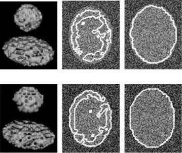
Now, we demonstrated the utility of image diffusion methods in our work. We take a synthetic 150 × 150 × 150 image volume composed of a sphere with a radius of 30 and an ellipsoid with axes 45, 60, and 30 inside a uniform noise specified by the image intensity range 0–150.

Figure 7.13 shows the result for steps (1)–(4) in Section 7.5, applied to this volume after Gaussian diffusion (Fig. 7.13(a)), and anisotropic diffusion

Figure 7.13: (a) Result for steps (1)–(4) with Gaussian diffusion. ( b) Cross sections of (a) for slice 40. (c) Cross section of final solution for slice 40. (d) Result for steps (1)–(4) with anisotropic diffusion. (e) Cross sections of (d) for slice 40. (f ) Cross section of final solution when using anisotropic diffusion (slice 40).

(Fig. 7.13(d)) defined by the equation:

where the threshold K can be determined by a histogram of the gradient magnitude. It was set to K = 300 in this example. The number of interactions of the numerical scheme used [52] to solve this equation was 4.

Figures 7.13( b) and (e) show the cross section corresponding to the slice 40. We observe that with anisotropic diffusion (Fig. 7.13(e)), the result is closer to the boundary than with the Gaussian one (Fig. 7.13( b)).

Also, the final result is more precise when preprocessing with anisotropic diffusion (Fig. 7.13(f )). This is expected because, according to Section 7.8, Eq. (7.45) enables the blurring of small discontinuities (gradient magnitude below K ) as well as enhancement of edges (gradient magnitude above K ).

Another point becomes clear in this example: The topological abilities of T-surfaces enable the correction of the defects observed in the surface extracted through steps (1)–(4). We observed that, after few interactions, the method gives two closed components. Thus, the reconstruction becomes better.

The T-surface parameters used are: c = 0.65, k = 1.32, and γ = 0.01. The grid resolution is 5 × 5 × 5, freezing point is set to 15, and threshold T (120, 134) in Eq. (7.12). The number of deformation steps for T-surfaces was 17. The model evolution can be visualized in http://virtual01.lncc.br/ rodrigo/tese/elipse.html.

7.9.2 Artery Reconstruction

This section demonstrates the advantages of applying T-surfaces plus isosurface methods. Firstly, we segment an artery from an 80 × 86 × 72 image volume obtained from the Visible Human project. This is an interesting example because the intensity pattern inside the artery is not homogeneous.

Figure 7.14(a) shows the result of steps (1)–(4) when using T (28, 32) to define the object characteristic function (Eq. (7.27)). The extracted topology is too different from that of the target. However, when applying T-surfaces the obtained geometry is improved.

Figure 7.14( b) shows the result after the first step of evolution. The merges among components improve the result. After four interactions of the