

Kluwer - Handbook of Biomedical Image Analysis Vol
.1.pdf
506 Farag, Ahmed, El-Baz, and Hassan
9.4.4.5 |
Cluster Prototype Updating |
|
|
|
|
|
|
|
|
|
|
|||||||||||||||
Taking the derivative of Fm w.r.t. vi and setting the result to zero, we have |
||||||||||||||||||||||||||
|
|
|
|
|
|
|
|
|
|
|
|
(yr − βr − vi) |
= |
|
||||||||||||
k |
N |
1 uikp (yk − βk − vi) + k |
N |
1 uikp |
|
α |
|
|
|
|
|
|||||||||||||||
= |
= |
|
NR |
yr Nk |
|
= 0. (9.41) |
||||||||||||||||||||
|
|
|
|
|
|
|
|
|
|
|
|
|
|
|
|
|
|
vi |
|
vi |
||||||
Solving for vi, we have |
|
|
|
|
|
|
|
|
|
|
|
|
|
|
|
|
|
|
|
|
|
|||||
|
|
|
N |
|
up |
(yk |
− |
βk) |
+ |
|
α |
|
|
(yr |
− |
βr ) |
|
|
||||||||
|
|
vi = |
|
= |
|
|
N |
|
|
p |
N |
|
(9.42) |
|||||||||||||
|
|
k |
1 |
|
|
|
|
|
|
|
|
|
k |
. |
||||||||||||
|
|
|
|
|
ik |
|
|
|
|
|
|
|
|
NR |
|
yr |
|
|
|
|
|
|
||||
|
|
|
|
|
|
|
|
|
(1 |
+ |
α) |
|
|
|
u |
|
|
|
|
|
|
|
|
|||
|
|
|
|
|
|
|
|
|
|
|
|
|
k=1 |
ik |
|
|
|
|
|
|
||||||
9.4.4.6 Bias Field Estimation
In a similar fashion, taking the derivative of Fm w.r.t. βk and setting the result to
zero we have |
|
|
|
|
|
|
|
|
|
|
|
|
|
|
|
|
|
|
|
|
|
|
|
|
|
|
|
|
|
|
|
= |
|
|
|
|
|
||||
i |
c |
|
∂ |
|
N |
|
|
|
|
βk β |
|
|
|
|||||||
1 |
∂βk |
k 1 uikp (yk − βk − vi)2 |
= 0. |
(9.43) |
||||||||||||||||
|
= |
|
|
|
|
= |
|
|
|
|
|
|
|
|
k |
|
|
|
|
|
Since only the kth term in the second summation depends on βk, we have |
||||||||||||||||||||
|
|
|
|
|
|
|
− βk − vi)2 βk |
= |
|
|
|
|
|
|
||||||
i |
c |
|
|
∂ |
|
|
|
|
|
|
|
|
|
|||||||
|
1 |
∂βk |
uikp (yk |
|
|
β |
= 0. |
(9.44) |
||||||||||||
|
= |
|
|
|
|
|
|
|
|
|
|
|
|
k |
|
|
|
|
|
|
Differentiating the distance expression, we obtain |
|
|
|
|
|
|
|
|||||||||||||
yk |
|
|
|
|
|
|
|
|
|
|
βk |
= |
|
|
|
|
||||
c |
|
uikp |
|
|
c |
uikp |
c |
uikp vi |
|
|
|
|
|
|||||||
i |
1 |
− βk |
i 1 |
− i 1 |
|
β |
= 0. |
(9.45) |
||||||||||||
|
= |
|
|
|
|
|
|
= |
|
= |
|
|
|
|
|
|
|
k |
|
|
Thus, the zero-gradient condition for the bias field estimator is expressed as
|
|
|
c |
up vi |
|
|
β |
yk |
|
i=1 |
ik |
. |
(9.46) |
|
|
|||||
|
= |
= |
p |
|
|
|
|
|
c |
|
|
||
k |
− i |
1 uik |
|
|
||
9.4.4.7 BCFCM Algorithm
The BCFCM algorithm for correcting the bias field and segmenting the image into different clusters can be summarized in the following steps:
Step 1. Select initial class prototypes {vi}ic=1. Set {βk}kN=1 to equal and very small values (e.g. 0.01).
Step 2. Update the partition matrix using Eq. 9.40.

508 |
Farag, Ahmed, El-Baz, and Hassan |
(a) |
(b) |
(c) |
(d) |
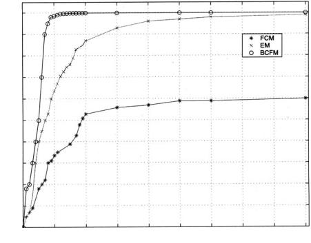
Figure 9.15: Comparison of segmentation results on a synthetic image corrupted by a sinusoidal bias field. (a) The original image, (b) FCM results, (c) BCFCM and EM results, and (d) bias field estimations using BCFCM and EM algorithms: this was obtained by scaling the bias field values from 1 to 255.
using either BCFCM or EM is presented in Fig. 9.15(d). This image was obtained by scaling the values of the bias field from 1 to 255. Although the BCFCM and EM algorithms produced similar results, BCFCM was faster to converge to the correct classification, as shown in Fig. 9.16.
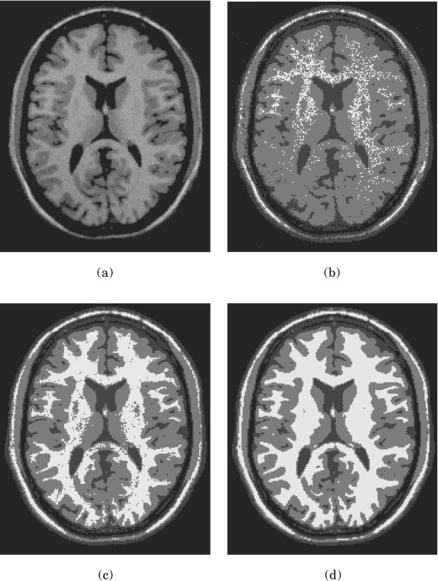
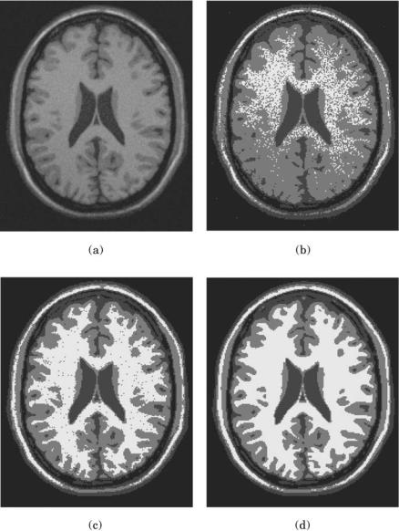
Figures 9.17 and 9.18 present a comparison of segmentation results between FCM, EM, and BCFCM, when applied on T1 weighted MR phantom corrupted with intensity inhomogeneity and noise. From these images, we can see that

512 |
Farag, Ahmed, El-Baz, and Hassan |
Table 9.2: Segmentation accuracy of different methods when applied on MR simulated data
|
|
|
SNR |
|
Segmentation Method |
13 db |
10 db |
8 db |
|
|
|
|
|
|
FCM |
98.92 |
86.24 |
78.9 |
|
EM |
99.12 |
93.53 |
85.11 |
|
BCFCM |
99.25 |
97.3 |
93.7 |
|
|
|
|
|
|
Figure 9.19 shows the results of applying the BCFCM algorithm to segment a real axial-sectioned T1 MR brain. Strong inhomogeneities are apparent in the image. The BCFCM algorithm segmented the image into three classes corresponding to background, GM, and WM. The bottom right image shows the estimate of the multiplicative gain, scaled from 1 to 255.
Figure 9.20 shows the results of applying the BCFCM for the segmentation of noisy brain images. The results using traditional FCM without considering the neighborhood field effect and the BCFCM are presented. Notice that the BCFCM segmentation, which uses the the neighborhood field effect, is much less fragmented than the traditional FCM approach. As mentioned before, the relative importance of the regularizing term is inversely proportional to the SNR of MRI signal. It is important to note, however, that the incorporation of spatial constraints into the classification has the disadvantage of blurring some fine details. There are current efforts to solve this problem by including contrast information into the classification. High contrast pixels, which usually represent boundaries between objects, should not be included in the neighbors.
9.5 Level Sets
The mathematical foundation of deformable models represents the confluence of physics and geometry. Geometry serves to represent object shape and physics puts some constrains on how it may vary over space and time. Deformable models have had great success in imaging and computer graphics. Deformable models include snakes and active contours. Snakes are used based on the geometric properties in image data to extract objects and anatomical structures in medical imaging. After initialization, snakes evolve to get the object. The change of

