Kluwer - Handbook of Biomedical Image Analysis Vol

to define diagonal coefficients

ci, j = ni, j + wi, j + si, j + ei, j + mi, j h2.

If we define right-hand sides at the nth discrete time step by

ri, j = mi, j h2uin,−j 1,

then for DF node corresponding to couple (i, j) we get the equation

ci, j un i, j − ni, j un i+1, j − wi, j un i, j−1 − si, j un i−1, j − ei, j un i, j+1 = ri, j . (11.28)

Collecting these equations for all DF nodes and taking into account Dirichlet boundary conditions, we get the linear system to be solved.

We solve this system by the so-called SOR (successive over relaxation) iterative method, which is a modification of the basic Gauss–Seidel algorithm

(see e.g. [46]). At the nth discrete time step we start the iterations by setting uin,(0)j = uin,−j 1, i = 1, . . . , m1, j = 1, . . . , m2. Then in every iteration l = 1, . . . and for every i = 1, . . . , m1, j = 1, . . . , m2, we use the following two-step procedure:

uin,(jl) = uin,(jl−1) + ω(Y − uin,(jl−1)).

The iterative process is stopped if R(l) < TOL R(0). Since the computing of residuum is time consuming itself, we check it, e.g., after every ten iterations. The relaxation parameter ω is chosen by a user to improve convergence rate of the method; we have very good experience with ω = 1.85 for this type of problems. Of course, the number of iterations depends on the chosen precision TOL, length of time step τ , and a value of the regularization parameter ε also plays a role. If one wants to weaken this dependence, more sophisticated approaches can be recommended (see e.g. [25, 35, 46] and paragraph below) but their implementation needs more programming effort. The semi-implicit co-volume method as presented above can be implemented in tens of lines.

We also outline shortly further approaches for solving the linear systems given in every discrete time step by (11.23). The system matrix has known (penta-diagonal) structure and moreover it is symmetric and diagonally dominant M-matrix. One could apply direct methods as Gaussian elimination, but this approach would lead to an immense storage requirements and computational effort. On the contrary, iterative methods can be applied in a very efficient way. In the previous paragraph we have already presented one of the most popular iterative methods, namely SOR. This method does not need additional storage, the matrix elements are used only to multiply the old solution values and convergence can be guaranteed for our special structure and properties of the system matrix . However, if the convergence is slow due to condition number of the system matrix (which increases with number of unknowns and for increasing τ and decreasing ε), faster iterative methods can be used. For example, the preconditioned conjugate gradient methods allow fast convergence, although they need more storage. If the storage requirements are reduced, then they can be very efficient and robust [25, 35]. For details of implementation of the efficient preconditioned iterative solvers for co-volume level set method, we refer to [25], cf. also [51]. Also an alternative direct approach based on operating splitting schemes can be recommended [57, 58].

In the next section, comparing CPU times, we will show that semi-implicit scheme is much more efficient and robust than explicit scheme for this type of problems. The explicit scheme combined with finite differences in space is

all considerations can be changed accordingly. We prefer the above definition of spatial discretization step, because it is closer to standard approaches to numerical solution of PDEs.

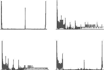
First we give some CPU times overview of the method. Since we are interested in finding a “steady state” (see discussion in Section 11.2) of the evolution in order to stop the segmentation process, the important properties are the number of time steps needed to come to this “equilibrium” and a CPU time for every discrete time step. We discuss CPU times in the experiment related to segmentation of the circle with a gap given in Fig. 11.12 (left), computed using

ε = 10−2 (see Fig. 11.14 (top left)). The testing image has 200 × 200 pixels and the computational domain corresponds to the whole image domain. Since for the boundary nodes we prescribe Dirichlet boundary conditions, we have

M = 198 × 198 degrees of freedom. As the criterion to recognize the “steady state,” we use a change in L2 norm of solution between subsequent time steps, i.e., we check whether

@

h2 (unp − unp−1)2 < δ

p

with a prescribed threshold δ. For the semi-implicit scheme and small ε (then the downwards motion of the “steady state” is very slow) a good choice of threshold is δ = 10−5.

Reasonable time steps for our semi-implicit method are of order (10h)2, e.g., for the discussed example very good results regarding CPU times and precision have been obtained for τ [0.001, 0.01]. Since by a classical criterion the precision of numerical schemes for parabolic equations is optimal for τ ≈ h2, we have also computed such a case. But, no significant difference due to precision has been observed, only much longer CPU time was necessary. In our example

τ = 5 × 10−3 and 20 time steps yield the segmentation result (using threshold

δ = 10−5). On 2.4 GHz Linux PC, the overall CPU time for this segmentation was 4.93 sec (i.e., approximately 0.25 sec for one time step including construction of coefficients and solving the linear system). This CPU time was obtained with TOL = 10−3. Since we are mainly interested in “equilibrium,” one can also decide that such precision is not necessary in every discrete time step. With increasing TOL fewer numbers of SOR iterations are needed. Another way is to prescribe a fixed number (but not too small) of iterations in every time step, e.g., ten

612 Mikula, Sarti, and Sgallari

inner edges of the circle) are given by two large gaps in histogram. In the top right there is a histogram of the segmentation function given by the explicit scheme after 500 time steps, and then after 1000 (bottom left) and 5000 (bottom right) time steps. We see that, due to necessity of small time step, the formation of the piecewise flat solution is very slow for explicit scheme. Although after 1000 time steps one can see the formation of two gaps which could be already used for detection of “final” segmentation result, the CPU time for 1000 steps of explicit scheme is 49.5 sec, which is ten times longer than for semi-implicit scheme. If we would like to obtain a similar histogram as plotted in the top left using an explicit scheme, we would need 100 times longer CPU time as in the case of semi-implicit scheme.

experiments without noise there is no significant difference by changing K . We get the same behavior of the method changing K from 0.1 to 10. It is understandable because the function g plays a role only along edges and its more (K > 1) or less (K < 1) quickly decreasing profile governs only speed by which level sets of solution are attracted to the edge from a small neighborhood. Everywhere else only pure mean curvature motion is considered (g = 1).

The situation is different for noisy images, e.g., depicted in Fig. 11.12 (right) and Figs. 11.16 and 11.17. The extraction of the circle in noisy environment takes a longer time (200 steps with τ = 0.01 and K = 1) and it is even worse for K = 10. However, decreasing the parameter K gives stronger weight to mean curvature flow in noisy regions, so we can extract the circle fast, in only 20 steps with the same τ = 0.01. In the case of noisy images, also the convolution plays a role. For example, if we switch off the convolution, the process is slower. But decreasing

K can again improve the speed of segmentation process. In our computations we either do not apply convolution to I0 or we use image presmoothing by m × m

pixel mask with weights given by the Gauss function normalized to unit sum.

We start all computations with initial function given as a peak centered in a “focus point” inside the segmented object, as plotted, e.g., in Fig. 11.10 (top left). Such a function can be described for a circle with center s and radius

can be subtracted from the peak-like profile. If the computational domain

corresponds to image domain, we use R = 0.5. For small objects a smaller R

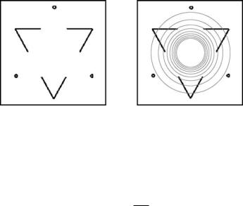
Figure 11.20: Image with subjective contours: double-Kanizsa triangle (left), and image together with isolines of initial segmentation function (right) (color slide).

can be used to speed up computations. Our choice of peak-like initial function is motivated by its nearly flat profile near the boundary of computational domain. However, other choices, e.g., u0(x) = 1 − , are also possible. If we put the focus point s not too far from the center of mass of the segmented object, we get only slightly different evolution of the segmentation function and same segmentation result.

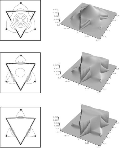
Now we will discuss some further segmentation examples. In Fig. 11.20 we present image (234 × 227 pixels) with subjective contours of the classic triangle of Kanizsa. The phenomenon of contours that appear in the absence of physical gradients has attracted considerable interest among psychologists and computer vision scientists. Psychologists suggested a number of images that strongly require image completion to detect the objects. In Fig. 11.20 (left), two solid triangles appear to have well defined contours, even in completely homogeneous areas. Kanizsa called the contours without gradient “subjective contours” [29], because the missed boundaries are provided by the visual system of the subject. We apply our algorithm in order to extract the solid triangle and complete the boundaries. In Figs. 11.21 and 11.22 we present evolution of the segmentation function together with plots of level lines accumulating along edges and closing subjective contours areas. In this experiment we used ε = 10−5, K = 1, v = 0.5,

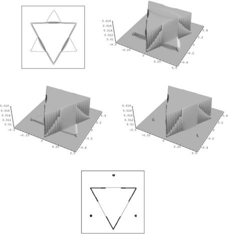
τ = 0.001, TOL = 10−3. For long time periods (from 60th to 300th time step) we can also easily detect subjective contours of the second triangle. The first one, given by closing of the solid interrupted lines, is presented in Fig. 11.22 (bottom), visualizing level line (min(u) + max(u))/2. Interestingly, for bigger ε the second triangle has not been detected.

Figure 11.21: Level lines (left) and graphs of the segmentation function (right) in time steps 10, 30, and 60 (color slide).

Figure 11.22: Level lines and graph of the segmentation function in time step 100 (top row). Then we show graphs of segmentation function after 300 and 800 steps (middle row). In the bottom row we plot the segmented Kanizsa triangle (color slide).

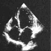
The next examples are related to medical image segmentation. First we process a 2D echocardiography (165 × 175 pixels) with high level of noise and gaps in ventricular and atrium boundaries (see Fig. 11.23).

In Fig. 11.24 we present segmentation of the left atrium. We start with peaklike segmentation function, v = 1, and we use ε = 10−2, K = 0.1, τ = 0.001, TOL = 10−3, and δ = 10−5. In the top row of the figure we present the result of segmentation with no presmoothing of the given echocardiography. In such a case 68 time steps, with overall CPU time of 6.54 sec, were needed for threshold δ.

Figure 11.23: Echocardiographic image with high level of noise and gaps.

In the top right we see a graph of the final segmentation function. In the middle row we see its histogram (left) and zoom of the histogram around max(u) (right). By that we take level 0.057 for visualization of the boundary of segmented object (top left). In the bottom row we present the result of segmentation using 5 × 5 convolution mask. Such a result is a bit smoother and 59 time steps (CPU time = 5.65 sec) were used.

For visualization of the segmentation level line in further figures, we use the same strategy as above, i.e. the value of u just below the last peak of histogram (corresponding to upper “flat region”) is chosen. In segmentation of the right atrium, presented in Fig. 11.25, we took the same parameters as above and no presmoothing was applied. CPU time for 79 time steps was 7.59 sec. In segmentation of the left and right ventricles, with more destroyed boundaries, we use

K = 0.5 and we apply 5 × 5 convolution mask (other parameters were same as above). Moreover, for the left ventricle we use double-peak-like initial function (see Fig. 11.26 (top)) to speed up the process for such highly irregular object. In that case 150 time steps (CPU time = 14.5 sec) were used. For the right ventricle, 67 time steps (CPU time = 6.57 sec) were necessary to get segmentation result, see Fig. 11.27.

In the last example given in Fig. 11.28, we present segmentation of the mammography (165 × 307 pixels). Without presmoothing of the given image and with parameters ε = 10−1, K = 0.1, τ = 0.0001, v = 1, TOL = 10−3, and δ = 10−5 we get the segmentation after 72 time steps. Since there are no big gaps, we take larger ε and since the object is small (found in a shorter time) we use smaller time step τ .