Kluwer - Handbook of Biomedical Image Analysis Vol

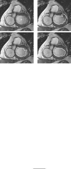
Figure 10.21: Heart MRI image. Top row: initial snakes and standard geometric snakes. Bottom row: GGVF snakes and final RAGS snakes showing improvement on the top right of the left snake and the lower region of the right snake.

dard snake leaks out of the object, similar to the effect demonstrated with the synthetic image in Fig. 10.15.

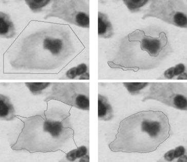
10.9.5 Results on Color Images

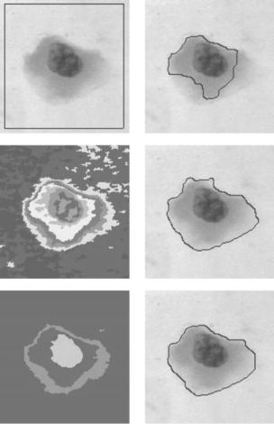
We now consider the performance of the RAGS snake on color images. In Fig. 10.23 we can see a cell image with both strong and fuzzy region boundaries. Note how the fuzzy boundaries to the right of the cell “dilute” gradually into the background. So the results in the top-right image again demonstrate an example of weak-edge leakage, similar to the example in Fig. 10.22, where the standard geometric snake fails to converge on the outer boundary. The middle and bottom rows show the converged RAGS snake using the oversegmentation and undersegmentation color region maps produced by the mean shift algorithm.

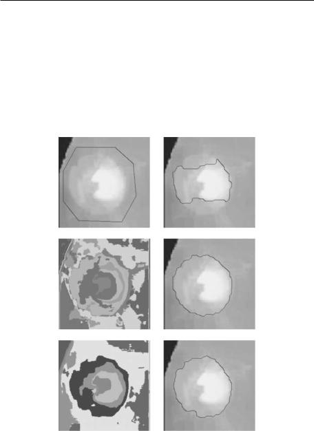
A very similar example is demonstrated in Fig. 10.24 in application to images of the optic disk in which the blood vessels have been removed using color mathematical morphology techniques. Again, the failing performance of the standard

Figure 10.22: Heart MRI image. Top row: initial snake, and standard geometric snake. Bottom row: GGVF snake and final RAGS snake showing better convergence and no leakage (original image courtesy of GE Medical Systems).

snake is shown along with the RAGS results on both oversegmentation and undersegmentation regions.

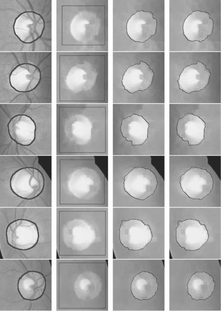
In Fig. 10.25, a full application of RAGS is presented where the resulting regions from the RAGS snake are quantitatively evaluated against those hand-labeled by an expert ophthalmologist. The first column represents these groundtruth boundaries. The second column shows the position of the starting RAGS snakes. The boundary of the optic disk is quite fuzzy and well blended with the background. The region force helps the proposed snake stop at weak edges while the standard geometric snake leaks through (as shown in Fig. 10.24) and the accuracy of the GGVF snake is highly dependent on where the initial snake is placed (hence GGVF snake results are not provided). The last two columns illustrate the RAGS results using oversegmented and undersegmented regions of the mean shift algorithm respectively.

A simple measure of overlap is used to evaluate the performance of the RAGS snake against its corresponding groundtruth:

M= n( A ∩ B) n( A B)

Figure 10.23: Weak-edge leakage testing. Top row: original image with starting contour and geodesic snake which steps through. Middle row: oversegmentation color region map and converged RAGS snake. Bottom row: undersegmentation color region map and converged RAGS snake (original image courtesy of Bristol Biomedical Image Archive, Bristol University, UK) (color slide).

where A and B correspond to ground-truth and RAGS localized optic disk regions respectively, and n(·) is the number of pixels in a region. Table 10.2 shows the result of measurement M demonstrating a 91.7% average performances for both over/undersegmentation RAGS respectively.

The final example in Fig. 10.26 shows a darker cell center compared to the cell outer region, but more significantlythe object of interest is surrounded by

map. The theory behind RAGS is standalone and hence the region force can be generated starting from any reasonable segmentation technique. We also showed its simple extension to color gradients. We demonstrated the performance of RAGS, against the standard geometric snake and the geometric GGVF snake, on weak edges and noisy images as well as on a number of other examples.

The experimental results have shown that the region-aided snake is much more robust toward weak edges. Also, it has better convergence quality compared with both the standard geometric snake and the geometric GGVF snake. The weak-edge leakage problem is usually caused by inconclusive edge values at the boundaries, which makes it difficult for gradient-based techniques to define a good edge. The gradual changes do not provide sufficient minima for the stopping function to prevent the level set accumulating in that area. The diffused region map gives the snake an extra underlying force at the boundaries. It also makes the snake more tolerable to noise as shown by the harmonic shape recovery experiment and many of the real images. The noise in the image introduces local minima in the stopping function preventing the standard geometric snake to converge to the true boundary. However, for RAGS the diffused region forces give a better global idea of the object boundary in the noise clutter and help the snake step closer and converge to the global minima.

10.11 Further Reading

Deformable contour models are commonly used in image processing and computer vision, for example for shape description [21], object localization [22], and visual tracking [23].

A good starting point to learn about parametric active contours is [24]. These snakes have undergone significant improvements since their conception, for example see the GVF snake in [7,9]. Region-based parametric snake frameworks have also been reported in [25–27]

The geometric model of active contours was simultaneously proposed by Caselles et al. [1] and Malladi et al. [2]. Geometric snakes are based on the theory of curve evolution in time according to intrinsic geometric measures of the image. They are numerically implemented via level sets, the theory of which can be sought in [15, 16].

There has been a number of works based on the geometric snake and level set framework. Siddiqi et al. [14] augmented the performance of the standard geometric snake that minimizes a modified length functional by combining it with a weighted area functional. Xu et al. extended their parametric GVF snake [7] into the generalized GVF snake, the GGVF, in [9]. Later, they also established an equivalence model between parametric and geometric active contours [10] using the GGVF. A geometric GGVF snake enhanced with simple region-based information was presented in [10]. Paragios et al. [28, 29] presented a boundary and region unifying geometric snake framework which integrates a region segmentation technique with the geometric snake. In [30], Yezzi et al. developed coupled curve evolution equations and combined them with image statistics for images of a known number of region types, with every pixel contributing to the statistics of the regions inside and outside an evolving curve. Using color edge gradients, Sapiro [6] extended the standard geometric snake for use with color images (also see Fig. 10.6). In [11], Chan et al. described a region-segmentation- based active contour that does not use the geometric snake’s gradient flow to halt the curve at object boundaries. Instead, this was modeled as an energy minimization of a Mumford–Shah-based minimal partition problem and implemented via level sets. Their use of a segmented region map is similar to the concept we have explored here.

Level set methods can be computationally expensive. A number of fast implementations for geometric snakes have been proposed. The narrow band technique, initially proposed by Chop [31], only deals with pixels that are close to the evolving zero level set to save computation. Later, Adalsterinsson et al. [32] analyzed and optimized this approach. Sethian [33, 34] also proposed the fast marching method to reduce the computations, but it requires the contours to monotonically shrink or expand. Some effort has been expended in combining these two methods. In [35], Paragios et al. showed this combination could be efficient in application to motion tracking. Adaptive mesh techniques [36] can also be used to speed up the convergence of PDEs. More recently, additive operative splitting (AOS) schemes were introduced by Weickert et al. [37] as an unconditionally stable numerical scheme for nonlinear diffusion in image processing. The basic idea is to decompose a multidimensional problem into one-dimensional ones. AOS schemes can be easily applied in implementing level set propagation [38].

φin−1, j )/ x, Di−, jy = (φin, j − φin, j−1)/ y are the forward and backward differences, respectively.

The external forces left in (10.17) contribute the third underlying static velocity field for snake evolution. Their direction and strength are based on spatial

position, but not on the snake. This motion can be numerically approximated

as follows. Let U (x, y, t) denote the underlying static velocity field according to

˜ − ·

β R g( ). We check the sign of each component of U and construct one-sided upwind differences in the appropriate (upwind) direction [16]:

=

where U (u, v). Thus, (10.17) is numerically solved using the schemes described above.

Questions

1.What are the advantages of geometric snakes over their parametric counterparts?

2.Which are some of the key papers on the geometric snake?

3.How do I diffuse the region segmentation map?

4.Describe how weighting functions p(·) and q(·) behave in vector diffusion?

5.What are the parameters in RAGS?

6.How do I choose the parameter values?

7.What are some of the disadvantages of RAGS?