

Kluwer - Handbook of Biomedical Image Analysis Vol
.1.pdfCo-Volume Level Set Method in Subjective Surface |
597 |
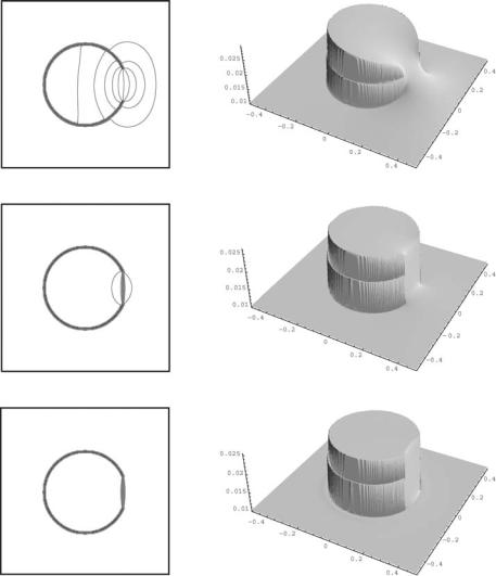
Figure 11.13: Experiment on testing image plotted in Fig. 11.12 (left). The results of evolution of the segmentation function (in the left its isolines, in the right its graphs) after 10 (top row) and 100 (bottom row) time steps. In this case,
ε = 1, the shape is stable, but moving downwards in a “self-similar” form, so it is not utilizable as the segmentation result.
very good segmentation results as presented in Fig. 11.14. Of course, smaller ε is needed to close larger gaps (see Fig. 11.15).
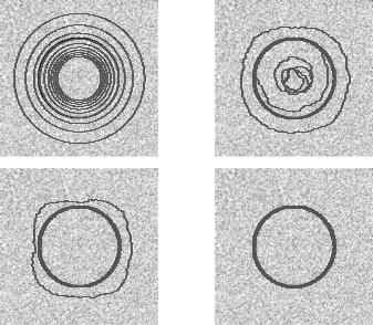
If there is a noisy image as in Fig. 11.12 (right), the motion of level lines to shock is more irregular, but finally the segmentation function is smoothed as well (see Figs. 11.16 and 11.17). If the regularization parameter ε is small, then piecewise flat profile of the segmentation function will move very slowly downwards, so it is easy to stop the evolution and get the result of segmentation process.
In the presented experiments, we have seen that the solution of Eq. (11.2) is well suited to finding and completing edges in (noisy) images. Its advection– diffusion mechanism leads to promising results. In the next section we give an efficient and robust computational method for its solution.

598 |
Mikula, Sarti, and Sgallari |
Figure 11.14: Results of the segmentation process for testing image plotted in Fig. 11.12 (left) using ε = 10−2 (top left) and ε = 10−5 (top right). The isoline (max (u) + min (u))/2 well represents the segmented circle (bottom red line). For large range of ε, we get satisfactory results (color slide).
11.3 Semi-implicit Co-Volume Scheme
We present our method in discretization of Eq. (11.8), although we always use its ε-regularization (11.2) with a specific ε > 0. The notation is simpler in the case of (11.8) and it will be clear where regularization appears in the numerical scheme.
First we choose a uniform discrete time step τ and a variance σ of the smoothing kernel Gσ . Then we replace time derivative in (11.8) by backward difference. The nonlinear terms of the equation are treated from the previous time step while the linear ones are considered on the current time level, this means semi-implicitness of the time discretization. In the last decade, semiimplicit schemes have become a powerful tool in image processing, we refer e.g. to [3, 4, 25–27, 33, 37, 51, 57, 58].
Semi-implicit in time discretization. Let τ and σ be fixed numbers, I0 be a given image, and u0 be a given initial segmentation function. Then, for
Co-Volume Level Set Method in Subjective Surface |
599 |
Figure 11.15: Segmentation of the circle with a big gap (Fig. 11.12 (middle)) using ε = 1 (top), ε = 10−2 (middle), and ε = 10−5 (bottom). For bigger missing part a smaller ε is desirable. In the left column we see how close to the edges the isolines are accumulating and closing the gap, and in the right we see how steep the segmentation function is along the gap (color slide).
600 |
|
|
Mikula, Sarti, and Sgallari |
|
|
|
|
|
|
|
|
|
|
|
|
|
|
|
|
|
|
|
|
|
Figure 11.16: Isolines of the segmentation function in the segmentation of the noisy circle (Fig. 11.12 (right)) are shown in time steps 0, 50, 100, and 200. Since the gap is not so big we have chosen ε = 10−1 (color slide).
n = 1, . . . , N, we look for a function un, solution of the equation,
| un−1 |
| |
τ |
= · |
|
| un−1 |
| |
|
|
|
1 |
|
|
un − un−1 |
|
g0 |
un |
|
. |
(11.11) |
|
|
|
|
|
|
|
|||
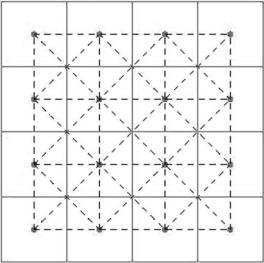
A digital image is given on a structure of pixels with rectangular shape, in general (red rectangles in Fig. 11.18). Since discrete values of I0 are given in pixels and they influence the model, we will relate spatially discrete approximations of the segmentation function u also to image pixels, more precisely, to their centers (red points in Fig. 11.18). In every discrete time step of the method (11.11), we have to evaluate gradient of the segmentation function at the previous step | un−1|. For that goal, it is reasonable to put a triangulation (dashed black lines in Fig. 11.18) inside the pixel structure and take a piecewise linear approximation of the segmentation function on this triangulation. Such an approach will give a constant value of the gradient per triangle, allowing simple and clear construction of fully discrete system of equations. This is the main feature of the co-volume [25, 56] and finite element [13–15] methods in solving mean curvature flow in the level set formulation.

Co-Volume Level Set Method in Subjective Surface |
601 |
40 |
|
|
|
120 |
|
|
|
|
|
|
|
|
|
|
|
|
|
|
|
100 |
|
|
|
30 |
|
|
|
80 |
|
|
|
|
|
|
|
|
|
|
|
20 |
|
|
|
60 |
|
|
|
|
|
|
|
|
|
|
|
|
|
|
|
40 |
|
|
|
10 |
|
|
|
20 |
|
|
|
|
|
|
|
|
|
|
|
0.015 |
0.02 |
0.025 |
0.03 |
0.015 |
0.02 |
0.025 |
0.03 |
Figure 11.17: The graph of the segmentation function and its histograms in time steps 100 and 200 for the same experiment as presented in Fig. 11.16. The histograms give a practical advise to shorten the segmentation process in case of noisy images. For a noisy image, the formation of completely piecewise flat subjective surface takes longer time. However, the gaps in histogram of the segmentation function are developed soon. It allows to take any level inside these gaps and to visualize the corresponding level line to get desirable segmentation result (color slide).
As can be seen in Fig. 11.18, in our method the centers of pixels are connected by a new rectangular mesh and every new rectangle is splitted into four triangles. The centers of pixels will be called degree of freedom (DF) nodes. By this procedure we also get further nodes (at crossing of red lines in Fig. 11.18) which, however, will not represent degrees of freedom. We will call them non-degree of freedom (NDF) nodes. Let a function u be given by discrete values in the pixel centers, i.e. in DF nodes. Then in additional NDF nodes we take the average value of the neighboring DF nodal values. By such defined values in NDF nodes, a piecewise linear approximation uh of u on the triangulation can be built. Let us note that we restrict further considerations in this chapter only to this type of grids. For triangulation Th, given by the previous construction, we construct a co-volume (dual) mesh. We modify a basic
602 |
Mikula, Sarti, and Sgallari |
Figure 11.18: The image pixels (red solid lines) corresponding to co-volume mesh. Triangulation (black dashed lines) for the co-volume method with degree of freedom nodes (red round points) corresponding to centers of pixels (color slide).
approach given in [25, 56] in such a way that our co-volume mesh will consist of cells p associated only with DF nodes p of Th, say p = 1, . . . , M. Since there will be one-to-one correspondence between co-volumes and DF nodes, without any confusion, we use the same notation for them. In this way we have excluded the boundary nodes (due to Dirichlet boundary data) and NDF nodes.
For each DF node p of Th, let C p denote the set of all DF nodes q connected to the node p by an edge. This edge will be denoted by σpq and its length by hpq . Then every co-volume p is bounded by the lines (co-edges) epq that bisect and are perpendicular to the edges σpq , q C p. By this construction, the covolume mesh corresponds exactly to the pixel structure of the image inside the computational domain where the segmentation is provided. We denote by Epq the set of triangles having σpq as an edge. In a situation depicted in Fig. 11.18, every Epq consists of two triangles. For each T Epq let cTpq be the length of the portion of epq that is in T, i.e., cTpq = m(epq ∩T), where m is a measure in IRd−1. Let Np be the set of triangles that have DF node p as a vertex. Let uh be a piecewise linear function on triangulation Th. We will denote a constant value

Co-Volume Level Set Method in Subjective Surface |
603 |
||
of | uh| on T Th by | uT | and define regularized gradients by |
|
||
| uT |ε = |
|
. |
|
ε2 + | uT |2 |
(11.12) |
||
We will use the notation up = uh(xp), where xp is the coordinate of the node p of triangulation Th.
With these notations, we are ready to derive co-volume spatial discretization. As is usual in finite volume methods [20, 34, 44], we integrate (11.11) over every
co-volume p, i = 1, . . . , M. We get |
|
|
|
| un−1| |
|
|
|
|
|
|||||||||||
p | un−1| |
τ |
|
= p · |
|
|
|
|
|
||||||||||||
1 |
|
un − un−1 |
dx |
|
|
|
g0 |
un |
|
|
dx. |
(11.13) |
||||||||
|
|
|
|
|
|
|
|
|
|
|
|
|||||||||
For the right-hand side of (11.13), using divergence theorem we get |
|
|||||||||||||||||||
|
p · |
| un−1| |
|
|
= ∂ p |
| un−1| |
∂ν |
|
||||||||||||
|
|
|
g0 |
un |
|
|
dx |
|
|
g0 |
∂un |
ds |
|
|||||||
|
|
|
|
|
|
|
|
|
|
|
|
|
||||||||
|
|
|
|
|
|
|
|
|
|
|
g0 |
|
|
∂un |
|
|||||
|
|
|
|
|
|
|
|
|
= q C p epq |
|
|
|
||||||||
|
|
|
|
|
|
|
|
|
|
|
|
ds. |
|
|||||||
|
|
|
|
|
|
|
|
|
| un−1| |
|
∂ν |
|
||||||||
|
|
|
|
|
|
|
|
|
|
|
|
|
|
|
|
|
|
|
|
|
So we have an integral formulation of (11.11)
|
1 |
|
un − un−1 |
dx |
|
g0 |
|
|
∂un |
ds |
(11.14) |
p | un−1| |
|
τ |
= q C p epq | un−1 |
| ∂ν |
|
||||||
|
|
|
|
|
|
|
|
|
|
|
|
expressing a “local mass balance” property of the scheme. Now the exact “fluxes” on the right-hand side and “capacity function” on the left-hand side (see e.g. [34]) will be approximated numerically using piecewise linear reconstruction of un−1 on triangulation Th. If we denote gT0 approximation of g0 on a triangle
T Th, then for the approximation of the right-hand side of (11.14), we get
|
|
|
|
|
|
|
|
|
|
cT |
|
gT0 |
|
|
uqn − unp , |
(11.15) |
|
q C p |
pq |
| |
un−1 |
| |
|
hpq |
|
|
T Epq |
T |
|
|
|
|
|||
and the left-hand side of (11.14) is approximated by
un |
− |
un−1 |
|
||
Mpm( p) |
p |
p |
, |
(11.16) |
|
|
τ |
|
|||
|
|
|
|
|
|
where m( p) is a measure in IRd of co-volume p and either
M |
|
|
1 |
|
, |
| |
un−1 |
| = |
|
m(T ∩ p) |
| |
un−1 |
| |
(11.17) |
p = |
un−1 |
|
|
m( p) |
||||||||||
|
| |
|
p |
T Np |
T |
|
||||||||
|
|
| |
p |
|
|
|
|
|
|
|
|
|
||
604 |
|
|
|
|
|
|
Mikula, Sarti, and Sgallari |
||
or |
|
|
|
|
|
|
|
|
|
M |
m(T ∩ p) |
|
|
1 |
|
|
(11.18) |
||
p = |
|
|
|
. |
|||||
m( p) |
| |
un−1 |
| |
||||||
|
|
|
|||||||
|
T Np |
|
|
T |
|
|
|||
The averaging of the gradients (11.17) has been used in [25, 56], and the approximation (11.18) is new and we have found it very useful regarding good convergence properties in solving the linear systems (see below) iteratively for
ε ' 1. Regularizations of both the approximations of the capacity function are as follows: either
|
Mpε |
= |
|
1 |
|
|
|
|
|
|
(11.19) |
|
|
n 1 |
|
|
|
|
|
|
|||
|
|
|
| |
u − |
|ε |
|
|
|
|
||
or |
|
|
p |
|
|
|
|
||||
|
|
|
|
|
|
|
|
|
|
|
|
Mε |
m(T ∩ p) |
|
|
|
1 |
|
|
(11.20) |
|||
= |
|
|
|
|
. |
||||||
p |
m( p) |
|
| |
un−1 |
|ε |
|
|||||
|
T Np |
|
|
|
|
T |
|
||||
Now we can define coefficients, where the ε-regularization is taken into account, namely,
bnp−1 |
= Mεpm( p), |
|
g0 |
|
|
(11.21) |
||
an−1 |
1 |
|
|
|
|
|
||
|
|
cT |
|
T |
|
, |
(11.22) |
|
pq |
= hpq |
pq |
| |
un−1 |
|ε |
|
||
|
|
|
T Epq |
T |
|
|||
which together with (11.15) and (11.16) give the following.
Fully-discrete semi-implicit co-volume scheme. Let u0p, p = 1, . . . , M, be given discrete initial values of the segmentation function. Then, for n =
1, . . . , N we look for unp, p = 1, . . . , M, satisfying
bnp−1unp + τ |
|
|
anpq−1(unp − uqn) = bnp−1unp−1. |
(11.23) |
q C p
Theorem. There exists a unique solution (un1 , . . . , unM ) of the scheme (11.23) for any τ > 0, ε > 0 and for every n = 1, . . . , N. Moreover, for any τ > 0, ε > 0 the following stability estimate holds
min |
0 |
min |
|
|
n |
max |
n |
max |
0 |
1 |
≤ n |
≤ N. |
(11.24) |
|||
p |
up ≤ |
p |
|
up ≤ |
|
p |
up ≤ |
|
p |
up, |
|
|
||||
Proof. The system (11.23) can be rewritten in the form |
|
|
||||||||||||||
|
|
|
|
|
|
|
|
|
|
|
|
|||||
bnp−1 + τ q |
|
C |
p |
anpq−1 |
unp − τ q |
C |
anpq−1uqn = bnp−1unp−1. |
(11.25) |
||||||||
|
|
|
|
|
|
|
|
|
p |
|
|
|
|
|
||
Co-Volume Level Set Method in Subjective Surface |
605 |
Applying Dirichlet boundary conditions, it gives the system of linear equations with a matrix, the off diagonal elements of which are symmetric and negative. Diagonal elements are positive and dominate the sum of absolute values of the nondiagonal elements in every row. Thus, the matrix of the system is symmetric and diagonally dominant M-matrix which imply that it always has a unique solution. The M-matrix property gives us the minimum–maximum principle, which can be seen by the following simple trick. We may temporarily rewrite (11.23) in the equivalent form
|
|
τ |
|
|
|
|
|
|
|
un |
+ n 1 |
an−1 |
(un |
− |
un) |
= |
un−1 |
(11.26) |
|
p |
pq |
p |
q |
p |
|
||||
|
|
bp− |
q C p |
|
|
|
|
|
|
|
|
|
|
|
|
|
|
|
|
and let max(un1 , . . . , unM ) be achieved in the node p. Then the second term on the left-hand side is non-negative and thus max(un1 , . . . , unM ) = unp ≤ unp−1 ≤ max(un1−1, . . . , unM−1). In the same way we can prove the relation for minimum and together we have
min un−1 |
≤ |
min un |
≤ |
max un |
≤ |
max un−1 |
, |
1 |
≤ |
n |
≤ |
N, |
(11.27) |
||||
p |
p |
p |
p |
p |
p |
p |
p |
|
|
|
|
|
|||||
which by recursion imply the desired stability estimate (11.24). |
|
||||||||||||||||
So far, we have said nothing about evaluation of gT0 included in coefficients (11.22). Since image is piecewise constant on pixels, we may replace the convolution by the weighted average to get Iσ0 := Gσ I0 (see e.g. [37]) and then relate discrete values of Iσ0 to pixel centers. Then, as above, we may construct its piecewise linear representation on triangulation and in such way we get constant value of Iσ0 on every triangle T Th. Another possibility is to solve numerically a linear heat equation for time t corresponding to variance σ with initial datum given by I0 (see e.g. [3]). The convolution represents a preliminary smoothing of the data. It is also a theoretical tool to have bounded gradients and thus a strictly positive weighting coefficient g0. In practice, the evaluation of gradients on discrete grid (e.g., on triangulation described above) always gives bounded values. So, working on discrete grid, one can also avoid the convolution, especially if preliminary denoising is not needed or not desirable. Then it is possible to work directly with gradients of piecewise linear representation of I0 in the evaluation of gT0 .
Our co-volume scheme in this paper is designed for the specific mesh (see Fig. 11.18) given by the rectangular pixel structure of 2D image. For simplicity of implementation and for the reader’s convenience, we will write the

606 |
Mikula, Sarti, and Sgallari |
co-volume scheme in a “finite-difference notation.” As is usual for 2D rectangular grids, we associate co-volume p and its corresponding center (DF node) with a couple (i, j), i will represent the vertical direction and j the horizontal direction. If is a rectangular subdomain of the image domain where n1 and n2 are number of pixels in the vertical and horizontal directions, respectively, then i = 1, . . . , m1, j = 1, . . . , m2, m1 ≤ n1 − 2, m2 ≤ n2 − 2 and M = m1m2. Similarly, the unknown value un p is associated with un i, j . For every co-volume p, the set Np consists of eight triangles (see Fig. 11.18). In every discrete time step n = 1, . . . , N, and for every i = 1, . . . , m1, j = 1, . . . , m2, we compute absolute value of gradient on these eight triangles denoted by Gik, j , k = 1, . . . , 8. For that goal, using discrete values of u from the previous time step, we use the following expressions (we omit upper index n − 1 on u):
Gi, j = ? |
0.5(ui, j |
+ |
+ |
+ |
h+ |
− |
ui, j |
− |
+ |
|
2 |
+ |
+ |
h− |
ui, j |
|
2 |
|
|||||||
|
, |
||||||||||||||||||||||||
1 |
|
|
|
|
|
|
1 |
|
ui 1, j 1 |
|
|
ui 1, j ) |
|
|
|
ui 1, j |
|
|
|
||||||
Gi, j = ? |
|
|
|
|
|
|
|
|
|
|
|
|
|
|
|
|
|
|
|
|
|
|
|
||
|
|
+ |
|
|
h |
|
− |
|
|
|
|
2 |
+ |
|
h |
|
|
, |
|||||||
2 |
|
|
|
|
|
|
0.5(ui, j |
|
ui+1, j −ui, j−1 ui+1, j−1 ) |
|
|
|
ui+1, j −ui, j |
|
|
|
|||||||||
Gi, j = ? |
|
|
|
|
|
|
|
|
|
|
|
|
|
|
|
|
|
||||||||
|
+ − + |
h |
− |
|
|
− |
|
|
2 |
+ |
|
−h |
|
|
, |
||||||||||
3 |
|
|
|
|
|
|
0.5(ui 1, j 1 ui+1, j |
|
ui, j−1 ui, j ) |
|
|
|
ui, j ui, j−1 |
|
|
|
|||||||||
Gi, j = ? |
|
|
|
|
|
|
|
|
|
|
|
|
|
|
|
|
|
|
|
|
|
||||
|
|
|
+ |
|
h |
|
|
|
|
|
|
2 |
+ |
|
h |
|
|
, |
|||||||
4 |
|
|
|
|
|
|
0.5(ui, j−1 ui, j −ui−1, j−1 −ui−1, j ) |
|
|
|
ui, j −ui, j−1 |
|
|
|
|||||||||||
Gi, j = ? |
|
|
|
|
|
|
|
|
|
|
|
|
|
|
|
|
|
|
|
|
|
|
|||
|
|
+ |
|
|
h |
|
|
|
|
|
|
2 |
+ |
|
h |
|
|
, |
|||||||
5 |
|
|
|
|
|
|
0.5(ui, j |
|
ui−1, j −ui, j−1 −ui−1, j−1 ) |
|
|
|
ui, j −ui−1, j |
|
|
|
|||||||||
|
|
|
|
|
|
|
|
|
|
|
|
|
|
|
|
|
|
|
|
|
|
|
|
|
|
Gi, j = ? |
0.5(ui, j |
+ |
+ |
− |
h+ |
− |
ui, j |
− |
− |
|
2 |
+ |
ui, j |
−h − |
|
2 |
|
||||||||
|
, |
||||||||||||||||||||||||
6 |
|
|
|
|
|
|
1 |
|
ui 1, j 1 |
|
|
ui 1, j ) |
|
|
|
ui 1, j |
|
|
|
||||||
Gi, j = ? |
|
|
|
|
|
|
|
|
|
|
|
|
|
|
|
|
|
|
|
|
|
||||
|
|
+ |
|
|
h |
|
|
|
|
|
|
2 |
+ |
|
h |
|
|
, |
|||||||
7 |
|
|
|
|
|
|
0.5(ui, j |
|
ui, j+1 −ui−1, j −ui−1, j+1 ) |
|
|
|
ui, j+1 −ui, j |
|
|
|
|||||||||
|
|
|
|
|
|
|
|
|
|
|
|
|
|
|
|
|
|
|
|
|
|
|
|
|
|
Gi, j = ? |
+ |
+ |
+ |
h+ |
− |
ui, j |
− |
|
+ |
|
2 |
+ |
ui, j |
+ h− |
ui, j |
|
2 |
|
|||||||
|
|
. |
|||||||||||||||||||||||
8 |
|
|
|
|
|
|
0.5(ui 1, j |
|
ui 1, j 1 |
|
|
ui, j 1 ) |
|
|
|
1 |
|
|
|
||||||
In the same way, but only in the beginning of the algorithm, we compute values Giσ,, jk, k = 1, . . . , 8, changing u by Iσ0 in the previous expressions, where
Iσ0 is a smoothed image as explained in the paragraph above. Then for every i = 1, . . . , m1, j = 1, . . . , m2 we construct (north, west, south, and east)