Kluwer - Handbook of Biomedical Image Analysis Vol

snakes with time is guided by differential equations. These equations are derived from the energy minimization concept to describe the change of snakes with time. The output obtained using snakes depends highly on the initialization. It was found that initial curve has to lie close to the final solution to obtain required results. The initialization is relatively easy in the case of 2D images but in the 3D case it is very difficult. Also the topology change of the solution needs a special regulation to the model.

Level sets were invented to handle the problem of changing topology of curves. The level sets has had great success in computer graphics and vision. Also, it was used widely in medical imaging for segmentation and shape recovery. It proved to have advantages over statistical approaches followed by mathematical morphology. In the following section we will give a brief overview on level sets and its application in image segmentation.

9.5.1 Level Set Function Representation

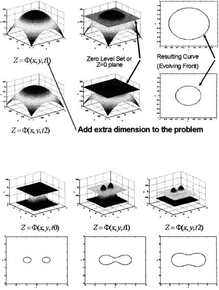
Level sets was invented by Osher and Sethian [52] to handle the topology changes of curves. A simple representation is that a surface intersects with the zero plane to give the curve. When this surfaces changes the curve changes. The surface can be described by the following equation:

φ(x, t) > 0 if x , φ(x, t) < 0 if x / , and φ(x, t) = 0 if x , (9.49)

where φ represents the surface function, denotes the set of points where the function is positive, and represents the set of points at which the function is zero. In Fig. 9.21, an example of a surface and its intersection with the zero plane is shown. This intersection is called the front. The surface changes with time, resulting in different fronts. So the level set function is positive at some points, negative at other points, and zero at the front . The time as extra dimension is added to the problem to track the changes of the front. The topology changes of the curve are handled naturally by this presentation as we see from Fig. 9.22. The first row represents the surface and the zero plane at different time samples and the second row represents the resulting curves. The front is initially two ellipses, then the two ellipses merge to make a closed curve and it changes and so on. This representation allows the front to merge and break.

Figure 9.21: Change of the level set function with time resulting in different

curves.

Figure 9.22: Topology change of curves with time.

9.5.2 Curve Evolution with Level Sets

To get an equation describing the change of the curve or the front with time, we will start with the asssumption that the level set function is zero at the front as follows:

Converting the terms to the dot product form of the gradient vector and the x and y derivatives vector, we get

Multiplying and dividing by | φ| and takeing the other part to be F, we get the following equation:

The selection of the speed function is very important to keep the change of the front smooth and also it is application dependent. Equation 9.55 represents speed function containing the mean curvature k. The positive sign means that the front is shrinking and the negative sign means that the front is expanding and is selected to be a small value for smoothness. The curvature term allows the front to merge and break and also handles sharp corners,

In 3D, the front will be an evolving surface rather than an evolving curve.

9.5.3 Stability and CFL Restriction

The numerical solution of the partial differential equation (PDE) describing the front is very important to be accurate and stable. For simplicity, Taylor’s series expansion is used to handle the partial derivatives of φ as listed below,

φxx(x, y, t) = (φ(x + 2)x, y, t) − 2φ(x, y, t) + φ(x − 2)x, y, t))/(2)x2),

(9.60)

φyy(x, y, t) = (φ(x, y + 2)y, t) − 2φ(x, y, t) + φ(x, y − 2)y, t))/(2)y2).

(9.61)

There are different numerical techniques used for this problem and the details are given in [52]. The solution is very sensitive to the time step. Time step is selected based on the Courant–Friedrichs–Levy (CFL) restriction. It requires the front to cross no more than one grid cell at each time step )t. This calculation will give the maximum time step that guarantees stability. From Eq. 9.62, we maximize the denominator and minimize the nominator to get the best value of the time step. The time step is calculated at each iteration of the process to maintain the stability of the solution:

9.5.4 Tracking the Front

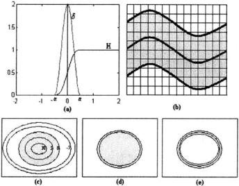
Now, the solution is to find the front iteratively at different time steps. We get the front by intersecting the surface with the zero plane. We need to track this front by getting the length of the front or getting the area enclosed. This information is very important in the segmentation problem as we will see in the next sections. Simply the enclosed area contains all the points at which the level set function is greater than or equal to zero and the points of the front are the points at which the level set function is zero. Applying the heaviside step and delta functions is very useful in getting the area and the front respectively. For numerical implementation, it is desirable to replace the heaviside and the delta functions by some counterparts. Approximations of these two functions are used to handle smoothness problem as follows:

interested in the change of the front. It is not important to get the solution at points far away from the front, so the solution is important at the points near the front. The points (highlighted in Fig. 9.23(b)) are called the narrow band points. The change of the level set function at these points only is considered. Other points (outside the narrow band) are called the far away points and they are given large positive or large negative values to be out of interest (not processed), and it speeds up the iterations. The use of the delta function defined by Eq. 9.64 is very important to give the narrow band points.

9.5.6 Reinitialization

The existence of the front means that the level set function has positive and negative parts, then it has negative and positive values including zeroes. The level set function with this property is called a signed distance function. This property should be kept through the iterations in order not to lose the front. There are different solutions for this problem [54]. We will discuss only the solution introduced by Osher et al. [55]. It was proved that recomputing the level set function by solving Eq. 9.67 frequently enough will maintain the function as signed distance function:

∂t

where it contains the sign function sign. When the level set function is negative, the information flows one way and when it is positive, the information flows the other way. The net effect is to “straighten out” the level set function on either sides of the zero level set,

By solving this equation, the derivative of φ with respect to time will vanish resulting in Eq. 9.68. | φ| = 1 denotes the measure for signed distance function.

9.6Application: MRA Data Segmentation Using Level Sets

The human cerebrovascular system is a complex three-dimensional anatomical

structure. Serious types of vascular diseases such as carotid stenosis, aneurysm,

and vascular malformation may lead to brain stroke, which is the third leading cause of death and the main cause of disability. An accurate model of the vascular system from MRA data volume is needed to detect these diseases at early stages and hence may prevent invasive treatments. A variety of methods have been developed for segmenting vessels within MRA. One class of methods is based on a statistical model, which classifies voxels within the image volume into either vascular or nonvascular class for time-of-flight MRA [56]. Another class of segmentation is based on intensity threshold where points are classified as either greater or less than a given intensity. This is the basis of the isointensity surface reconstruction method [57–59]. This method suffers from errors due to image inhomogeneities in addition; the choice of the threshold level is subjective. An alternative to segmentation is axis detection known as skeletonization process, where the central line of the tree vessels is extracted based on the tubular shape of vessels [60]. Other approaches for MRA vessel segmentation are the manually defined seed locations for segmentation [61].

In this section, we use level set method for image segmentation to improve the accuracy of the vascular segmentation. This work is a supervised classification which means that the number of classes and the class distribution are assumed to be known. Usually, the class distribution is assumed to be Gaussian with known mean and variance. In [53], classes were assumed to be phases separated by interface boundaries where each class has its corresponding level set function. A set of functionals were developed with properties of regularity. The level set function representation depends on these functionals. Each class occupies certain areas (regions) in the image. The level set function is represented based on the regions i.e. it is positive inside the region, negative outside, and zero on the boundary. The classes have no common areas i.e., the intersection between classes is not allowed. The sum of lengths of the interfaces between the areas is taken in consideration. The functionals are dependent mainly on these properties and they are expected to have a local minimum which is the segmented image. The change of each level set is guided by two forces, the minimal length of interfaces which is the internal force and the homogeneous class distribution which is the external one.

A PDE guides the motion of each level set. This work saves the manual initialization of level set functions [62]. Bad initialization for these functions makes the segmentation fail. Automatic seed initialization is made for each slice of the volume by dividing the image into windows, and based on the gray

This solution represents the level set function variation with time. When the function approaches the steady state, it does not change. It has positive, negative, and zero parts. We are interested only in the positive parts. Each pixel in the positive parts belongs to the associated class of its function. By this representation, the level set function formulation allows breaking and merging fronts since Eq. 9.72 contains the curvature term which is considered to be a smoothing part.

9.6.2 Volume Segmentation Algorithm

Step 0: Initialize φi, i [1, c].

Step 1: t = t + 1.

Step 2: Update each function using Eq. 9.72.

Step 3: Solve Eq. 9.67 for each of n iterations to keep the signed distance function property.

Step 4: Smooth each function and remove noise.

Step 5: If steady state is not reached, then go to Step 1, else go to next slice.

Step 0 is very important since bad initialization leads to bad segmentation. Automatic seed initialization is used to speed up the process and it is also less sensitive to noise. Automatic seed initialization is to divide the image into nonoverlapped windows of predefined size. Then the average gray level is calculated and compared to the mean of each class to specify the nearest class it belongs to. A signed distance function is initialized to each window. The connectivity filter is applied to remove the nonvessel tissues. The filter exploits the fact that the vascular system is a tree-like structure.

9.6.3 Segmentation Quality Measurement

A 2D phantom is designed to simulate the MRA. This phantom image contains many circles with decreasing diameters such as the cerebrovascular tree shape which is a cone-shaped. Then using the level set segmentation algorithm with this image, we obtain a resultant image containing the vessels. The SA is measured by Eq. 9.48.

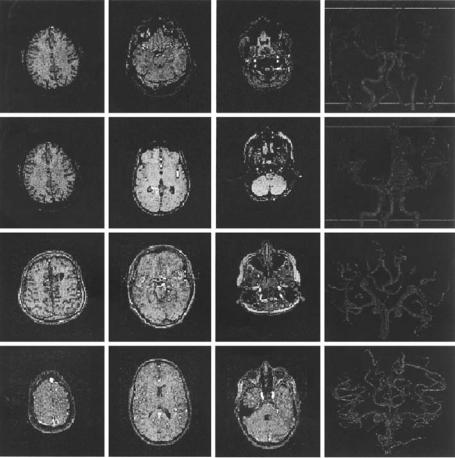
Figure 9.24: Segmentation and Visualization of different data sets.

9.6.4 Results and Discussion

The technique has been applied to different data sets of MR angiography phase contrast and time-of-flight types. For each type two volumes are used to prove the accuracy of the technique. The first type of data is 117 × 256 × 256 (the first two rows of Fig. 9.24) and the second type is 93 × 512 × 512 (the second two rows of Fig. 9.24). First, level sets are initialized by automatic seed initialization. Automatic seed initialization is used in each slice and each slice is divided into windows of size 5 × 5. An average mean is estimated for each class from the average histogram of the volume, and signed distance functions are assigned where each level set function is a collection of Gaussian surfaces added together with a