Kluwer - Handbook of Biomedical Image Analysis Vol

14 × 10−3

12

10

8

6

4

2

0

−2 0 50 100 150 200 250

y

Figure 9.9: 12 Gaussian components which are used in density estimation.

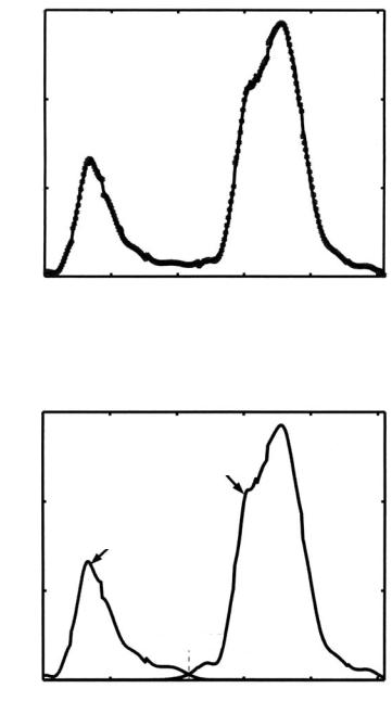
shows the estimated density for |ζ (y)|. Figure 9.9 shows all Gaussian components which are estimated after using dominant Gaussian components extracting algorithm and sequential EM algorithms. Figure 9.10 shows the estimated density for the CT slices shown in Figure 9.4. The Levy distance between the distributions Pes(y) and Pem(y) is 0.0021 which is smaller compared to the Levy distance between the distributions Pem(y) and P I(y).

Now we apply components classification algorithm on the ten Gaussian components that are estimated using sequential EM algorithm in order to determine which components belong to lung tissues and which components belong to chest tissues. The results of components classification algorithm show that the minimum risk equal to 0.004 48 occurs at threshold Th = 108 when Gaussian components 1, 2, 3, and 4 belong to lung tissues and component 5, 6, 7, 8, 9, and 10 belong to chest tissues. Figure 9.11 shows the estimated density for lung tissues and estimated density for chest and other tissues that may appear in CT.

The next step of our algorithm is to estimate the parameters for high-level process. A popular model for the high-level process is the Gibbs Markov mode, and we use the Bayes classifier to get initial labeling image. After we run Metropolis algorithm and GA to determine the coefficients of potential function E(x), we get

0.015

0.01

0.005

Figure 9.10: Estimated density for lung tissues and chest tissues.

0.015

p(q l2)

0.01

p(q l1)

0.005

Figure 9.11: Empirical density and estimated density for CT slice shown in

Fig. 9.4.

Figure 9.12: (a) Segmented lung using the proposed algorithm, error = 1.09%.

(b) Output of segmentation algorithm by selecting parameters for high-level process randomly, error = 1.86%. (c) Segmented lung by radiologist.

the following results: α = 1, θ1 = 0.89, θ2 = 0.8, θ3 = 0.78, θ4 = 0.69, θ5 = 0.54,

θ6 = 0.61, θ7 = 0.89 , θ8 = 0.56, and θ9 = 0.99.

The result of segmentation for the image shown in Fig. 9.4 using these parameters is shown in Fig. 9.12. Figure 9.12(a) shows the results of proposed algorithm. Figure 9.12(b) shows output of the Metropolis algorithm by selecting parameters randomly. Figure 9.12(c) shows the segmentation done by a radiologist.

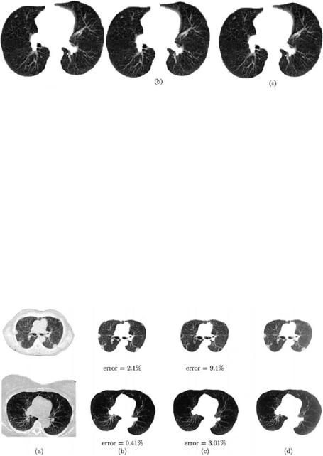
As shown in Fig. 9.12(a) the accuracy of our algorithm seems good if it is compared with the segmentation of the radiologist. Figure 9.13 shows comparison between our results and the results obtained by iterative threshold method which was proposed by Hu and Hoffman [23]. It is clear from Fig. 9.13 that the

Figure 9.13: (a) Original CT, (b) segmented lung using the proposed model, (c) segmented lung using the iterative threshold method, and (d) segmented lung by radiologist. The errors with respect to this ground truth are highlighted by red color.

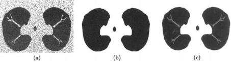
Figure 9.14: (a) Generated Phantom, (b) ground truth image (black pixel represent lung area, and gray pixels represent the chest area), and (c) segmented lung using the proposed approach (error 0.091). The errors with respect to this ground truth are highlighted by red color.

proposed algorithm segments the lung without causing any loss of abnormality tissues if it is compared with the iterative threshold method. Also, in order to validate our results we create a phantom which has the same distribution as lung and chest tissues. This phantom is shown in Fig. 9.14. One of the advantages of this phantom is that we know its ground truth. It is clear from Fig. 9.14 that the error between segmented lung and ground truth is small and this shows that the proposed model is accurate and suitable for this application.

9.4 Fuzzy Segmentation

As mentioned before, the objective of image segmentation is to divide an image into meaningful regions. Errors made at this stage would affect all higher level activities. Therefore, methods that incorporate the uncertainty of object and region definitions and the faithfulness of the features to represent various objects are desirable.

In an ideally segmented image, each region should be homogeneous with respect to some predicate such as gray level or texture, and adjacent regions should have significantly different characteristics or features. More formally, segmentation is the process of partitioning the entire image into c crisp maximally connected regions {Ri} such that each Ri is homogeneous with respect to some criteria. In many situations, it is not easy to determine if a pixel should belong to a region or not. This is because the features used to determine homogeneity may not have sharp transitions at region boundaries. To alleviate this situation, we can inset fuzzy set concepts into the segmentation process.

In fuzzy segmentation, each pixel is assigned a membership value in each of the c regions. If the memberships are taken into account while computing properties of regions, we oftain obtain more accurate estimates of region properties. One of the known techniques to obtain such a classification is the FCM algorithm [40, 41]. The FCM algorithm is an unsupervised technique that clusters data by iteratively computing a fuzzy membership function and mean value estimates for each class. The fuzzy membership function, constrained to be between 0 and 1, reflects the degree of similarity between the data value at that location and the prototypical data value, or centroid, ot its class. Thus, a high membership value near unity signifies that the data value at that location is close to the centroid of that particular class.

FCM has been used with some success in image segmentation in general [45, 46], however, since it is a point operation, it does not preserve connectivity among regions. Furthermore, FCM is highly sensitive to noise. In the following sections, we will present a new system to segment digital images using a modified Fuzzy c-means algorithm. Our algorithm is formulated by modifying the objective function of the standard FCM algorithm to allow the labeling of a pixel to be influenced by the labels in its immediate neighborhood. The neighborhood effect acts as a regularizer and biases the solution toward piecewise-homogeneous labelings. Such a regularization is useful in segmenting scans corrupted by scanner noise. In this paper, we will present the results of applying this algorithm to segment MRI data corrupted with a multiplicative gain field and salt and pepper noise.

9.4.1 Standard Fuzzy-C-Means

The standard FCM objective function for partitioning {xk}kN=1 into c clusters is given by

i=1 k=1

where {xk}kN=1 are the feature vectors for each pixel, {vi}ic=1 are the prototypes of the clusters and the array [uik] = U represents a partition matrix, U U, namely

setting them to zero results in two necessary but not sufficient conditions for

Jm to be at a local extrema. In the following subsections, we will derive these three conditions.

9.4.3.1 Membership Evaluation

The constrained optimization in Eq. 9.26 will be solved using one Lagrange multiplier

Solving for uik, we have

1

Substituting into Eq. 9.29, the zero-gradient condition for the membership estimator can be rewritten as

502 Farag, Ahmed, El-Baz, and Hassan

9.4.3.2 Cluster Prototype Updating

Using the standard Eucledian distance and taking the derivative of Fm w.r.t. vi

9.4.4 Application: Adaptive MRI Segmentation

In this section, we describe the application of the MFCM segmentation on MRI images having intensity inhomogeneity. Spatial intensity inhomogeneity induced by the radio frequency (RF) coil in magnetic resonance imaging (MRI) is a major problem in the computer analysis of MRI data [24–27]. Such inhomogeneities have rendered conventional intensity-based classification of MR images very difficult, even with advanced techniques such as nonparametric, multichannel methods [28–30]. This is due to the fact that the intensity inhomogeneities appearing in MR images produce spatial changes in tissue statistics, i.e. mean and variance. In addition, the degradation on the images obstructs the physician’s diagnoses because the physician has to ignore the inhomogeneity artifact in the corrupted images [31].

The removal of the spatial intensity inhomogeneity from MR images is difficult because the inhomogeneities could change with different MRI acquisition parameters from patient to patient and from slice to slice. Therefore, the correction of intensity inhomogeneities is usually required for each new image. In the last decade, a number of algorithms have been proposed for the intensity inhomogeneity correction. Meyer et al. [32] presented an edge-based segmentation scheme to find uniform regions in the image followed by a polynomial surface fit to those regions. The result of their correction is, however, very dependent on the quality of the segmentation step.

Several authors have reported methods based on the use of phantoms for intensity calibration. Wicks et al. [26] proposed methods based on the signal

produced by a uniform phantom to correct for MRI images of any orientation. Similarly, Tincher et al. [33] modeled the inhomogeneity function by a second-order polynomial and fitted it to a uniform phantom-scanned MR image. These phantom approaches, however, have the drawback that the geometry relationship of the coils and the image data is typically not available with the image data. They also require the same acquisition parameters for the phantom scan and the patient. In addition, these approaches assume the intensity corruption effects are the same for different patients, which is not valid in general [31].

The homomorphic filtering approach to remove the multiplicative effect of the inhomogeneity has been commonly used due to its easy and efficient implementation [29, 34]. This method, however, is effective only on images with relatively low contrast. Some researchers [33, 35] reported undesirable artifacts with this approach.

Dawant et al. [35] used operator-selected reference points in the image to guide the construction of a thin-plate spline correction surface. The performance of this method depends substantially on the labeling of the reference points. Considerable user interactions are usually required to obtain good correction results. More recently, Gilles et al. [36] proposed an automatic and iterative B- spline fitting algorithm for the intensity inhomogeneity correction of breast MR images. The application of this algorithm is restricted to MR images with a single dominant tissue class, such as breast MR images. Another polynomial surface fitting method [37] was proposed based on the assumption that the number of tissue classes, the true means, and standard deviations of all the tissue classes in the image are given. Unfortunately, the required statistical information is usually not available.

A different approach used to segment images with intensity inhomogeneities is to simultaneously compensate for the shading effect while segmenting the image. This approach has the advantage of being able to use intermediate information from the segmentation while performing the correction. Recently, Wells et al. [28] developed a new statistical approach based on the EM algorithm to solve the bias field correction problem and the tissue classification problem. Guillemaud et al. [38] further refined this technique by introducing the extra class “other.” There are two main disadvantages of this EM approach. First, the EM algorithm is extremely computationally intensive, especially for large

problems. Second, the EM algorithm requires a good initial guess for either the bias field or the classification estimate. Otherwise, the EM algorithm could be easily trapped in a local minimum, resulting in an unsatisfactory solution [31].

Another approach based on the FCM [40, 41] clustering technique has been introduced lately [42–44]. FCM has been used with some success in image segmentation in segmenting MR images [42, 47, 50]. Xu et al. [42] proposed a new adaptive FCM technique to produce fuzzy segmentation while compensating for intensity inhomogeneities. Their method, however, is also computationally intensive. They reduced the computational complexity by iterating on a coarse grid rather than the fine grid containing the image. This introduced some errors in the classification results and was found to be sensitive to a considerable amount of salt and pepper noise [43].

To solve the problem of noise sensitivity and computational complexity of the Pham and Prince method, we will generalize the MFCM algorithm to segment MRI data in the presence of intensity inhomogeneities.

9.4.4.1 Signal Modeling

The observed MRI signal is modeled as a product of the true signal generated by the underlying anatomy and a spatially varying factor called the gain field:

where Xk and Yk are the true and observed intensities at the kth voxel, respectively, Gk is the gain field at the kth voxel, and N is the total number of voxels in the MRI volume.

The application of a logarithmic transformation to the intensities allows the artifact to be modeled as an additive bias field [28]

where xk and yk are the true and observed log-transformed intensities at the kth voxel, respectively, and βk is the bias field at the kth voxel. If the gain field is known, it is relatively easy to estimate the tissue class by applying a conventional intensity-based segmenter to the corrected data. Similarly, if the tissue classes are known, we can estimate the gain field, but it may be problematic to estimate