Kluwer - Handbook of Biomedical Image Analysis Vol

This defines a system of linear equations in the expansion coefficients Cijk(r) that can be solved using standard techniques from numerical analysis, see Eqs. (8.21) and (8.23).

Equations (8.20a) and (8.20b) can then be conveniently expressed as

q

where A is a diagonal matrix, and b, c are vectors. In this equation we have also introduced the compact index notations p ≡ (i, j, k, r) and q ≡ (l, m, n, s) defined as

Next the matrix equation Ac = b must be solved for the vector c of dimension ( ) + D − 1, where N is the order of the expansion in Eq. (8.16) and D is the number of nonuniform input volumes. As is well known for many moving least-square problems, it is possible for the condition number of the matrix A to become very large. Any matrix is singular if its condition number is infinite

and can be defined as ill-conditioned if the reciprocal of its condition number approaches the computer’s floating-point precision. This can occur if the problem is overdetermined (number of sample points, xd greater than number of coefficients C) and underdetermined (ambiguous combinations of the coefficients C work equally well or equally bad). To avoid such numerical problems, a singular value decomposition (SVD) linear equation solver is recommended for use in combination with the moving least-squares method. The SVD solver identifies equations in the matrix A that are, within a specified tolerance, redundant (i.e., linear combinations of the remaining equations) and eliminates them thereby improving the condition number of the matrix. We refer the reader to [54] for a helpful discussion of SVD pertinent to linear least-squares problems.

Once we have the expansion coefficients c, we can readily express the Hessian matrix and the gradient vector of the combined input volumes as

evaluated at the moving expansion point x0. This in turn is used in Eq. (8.13) to compute the edge information needed to drive the level set surface.

8.4.1.3 Algorithm Overview

Algorithm 1 describes the main steps of our approach. The initialization routine, Algorithm 2, is called for all of the multiple nonuniform input volumes,

Vd. Each nonuniform input dataset is uniformly resampled in a common coordinate frame (V0’s) using trilinear interpolation. Edge information and the union,

V0, of the Vd’s are then computed. Algorithm 1 calculates Canny and 3D directional edge information using moving least-squares in a narrow band in each of the resampled input volumes, Vd, and buffers this in Vedge and Vgrad. Next Algorithm 1 computes the distance transform of the zero-crossings of the Canny edges and takes the gradient of this scalar volume to produce a vector field

Vedge, which pulls the initial level set model to the Canny edges. Finally the level set model is attracted to the 3D directional edges of the multiple input volumes,

Vgrad, and a Marching Cubes mesh is extracted for visualization. The level set

solver, described in Algorithm 3, solves Eq. (8.4) using the “up-wind scheme” (not explicitly defined) and the sparse-field narrow-band method of [36], with

V0 as the initialization and Vedge and Vgrad as the force field in the speed function.

Algorithm 1: MAIN(V1, . . . , VD )

comment: V1, . . . , VD are nonuniform samplings of object V

global V edge, V grad

Algorithm 2: INITIALIZATION(Vd)

comment: Preprocessing to produce good LS initialization

return (Vd)

Algorithm 3: SOLVELEVELSETEQ (V0, V, α, β)

comment: Solve Equation (8.4) with initial condition φ(t = 0) = V0

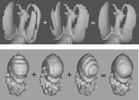
Figure 8.9: Nonuniform datasets merged to produce high-resolution level set models, (top) laser scan of a figurine and (bottom) MR scan of a mouse embryo.

volume dataset, and have the following resolutions: 26 × 128 × 128, 256 × 16 × 128, and 256 × 128 × 13. The last image in Fig. 8.9 presents the result produced by our multiscan segmentation method. The information in the first three scans has been successfully used to create a level set model of the embryo with a resolution of 256 × 128 × 130. The finer features of the mouse embryo, namely its hands and feet, have been reconstructed.

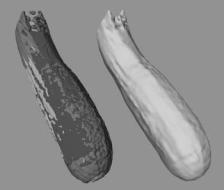
8.4.2.3 Zucchini Dataset

The final dataset consists of three individual MRI scans of an actual zucchini. The separate scans have been registered manually and are presented on the left side of Fig. 8.10, each with a different color. The resolutions of the individual scans are 28 × 218 × 188, 244 × 25 × 188, and 244 × 218 × 21. This image highlights the rough alignment of the scans. The right side of Fig. 8.10 presents the result of our level set segmentation. It demonstrates that our approach is able to extract a reasonable model from multiple datasets that are imperfectly aligned.

Figure 8.10: Three low-resolution MR scans of a zucchini that have been individually colored and overlaid to demonstrate their imperfect alignment. The level set model on the right is derived from the three low-resolution scans.

8.5 Segmentation of DT-MRI Brain Data

Diffusion tensor magnetic resonance imaging [55, 56] (DT-MRI) is a technique used to measure the diffusion properties of water molecules in tissues. Anisotropic diffusion can be described by the equation

∂t

where C is the concentration of water molecules and d is a diffusion coefficient, which is a symmetric second-order tensor

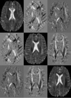
Figure 8.11 presents a “slice” of the diffusion tensor volume data of human brain used in our study. Each subimage presents the scalar values of the associated diffusion tensor component for one slice of the dataset.

Tissue segmentation and classification based on DT-MRI offers several advantages over conventional MRI, since diffusion data contains additional physical information about the internal structure of the tissue being scanned. However, segmentation and visualization using diffusion data is not entirely straightforward. First of all, the diffusion matrix itself is not invariant with respect to rotations, and the elements that form the matrix will be different for different

Figure 8.11: Slice of a tensor volume where every “element” of the image matrix corresponds to one component of the tensor D.

orientations of the sample or field gradient and therefore cannot themselves be used for classification purposes. Moreover, 3D visualization and segmentation techniques available today are predominantly designed for scalar and sometimes vector fields. Thus, there are three fundamental problems in tensor imaging: (a) finding an invariant representation of a tensor that is independent of a frame of reference, (b) constructing a mapping from the tensor field to a scalar or vector field, and (c) visualization and classification of tissue using the derived scalar fields.

The traditional approaches to diffusion tensor imaging involve converting the tensors into an eigenvalue/eigenvector representation, which is rotationally invariant. Every tensor may then be interpreted as an ellipsoid with principal axes oriented along the eigenvectors and radii equal to the corresponding eigenvalues. This ellipsoid describes the probabilistic distribution of a water molecule after a fixed diffusion time.

Using eigenvalues/eigenvectors, one can compute different anisotropy measures [55, 57–59] that map tensor data onto scalars and can be used for further

visualization and segmentation. Although eigenvalue/vector computation of the 3 × 3 matrix is not expensive, it must be repeatedly performed for every voxel in the volume. This calculation easily becomes a bottleneck for large datasets. For example, computing eigenvalues and eigenvectors for a 5123 volume requires over 20 CPU min on a powerful workstation. Another problem associated with eigenvalue computation is stability—a small amount of noise will change not only the values but also the ordering of the eigenvalues [60]. Since many anisotropy measures depend on the ordering of the eigenvalues, the calculated direction of diffusion and classification of tissue will be significantly altered by the noise normally found in diffusion tensor datasets. Thus it is desirable to have an anisotropy measure which is rotationally invariant, does not require eigenvalue computations, and is stable with respect to noise. Tensor invariants with these characteristics were first proposed by Ulug et al. [61]. In Section 8.5.1 we formulate a new anisotropy measure for tensor field based on these invariants.

Visualization and model extraction from the invariant 3D scalar fields is the second issue addressed in this chapter. One of the popular approaches to tensor visualization represents a tensor field by drawing ellipsoids associated with the eigenvectors/values [62]. This method was developed for 2D slices and creates visual cluttering when used in 3D. Other standard CFD visualization techniques such as tensor-lines do not provide meaningful results for the MRI data due to rapidly changing directions and magnitudes of eigenvector/values and the amount of noise present in the data. Recently Kindlmann [63] developed a volume rendering approach to tensor field visualization using eigenvalue-based anisotropy measures to construct transfer functions and color maps that highlight some brain structures and diffusion patterns.

In our work we perform isosurfacing on the 3D scalar fields derived from our tensor invariants to visualize and segment the data [64]. An advantage of isosurfacing over other approaches is that it can provide the shape information needed for constructing geometric models, and computing internal volumes and external surface areas of the extracted regions. There has also been a number of recent publications [65, 66] devoted to brain fiber tracking. This is a different and more complex task than the one addressed in this chapter and requires data with a much higher resolution and better signal-to-noise ratio than the data used in our study.

8.5.1 Tensor Invariants

Tensor invariants (rotational invariants) are combinations of tensor elements that do not change after the rotation of the tensor’s frame of reference, and thus do not depend on the orientation of the patient with respect to the scanner when performing DT imaging. The well-known invariants are the eigenvalues of the diffusion tensor (matrix) d, which are the roots of the corresponding characteristic equation

with coefficients

C1 = Dxx + Dyy + Dzz

C2 = Dxx Dyy − Dxy Dyx + Dxx Dzz − Dxz Dzx + Dyy Dzz − Dyz Dzy (8.28)

C3 = Dxx(Dyy Dzz − Dzy Dyz)

− Dxy(Dyx Dzz − Dzx Dyz) + Dxz(Dyx Dzy − Dzx Dyy).

Since the roots of Eq. (8.27) are rotational invariants, the coefficients C1, C2, and C3 are also invariant. In the eigen-frame of reference they can be easily expressed through the eigenvalues

and are proportional to the sum of the radii, surface area, and the volume of the “diffusion” ellipsoid. Then instead of using (λ1, λ2, λ3) to describe the dataset, we can use (C1, C2, C3). Moreover, since Ci are the coefficients of the characteristic equation, they are less sensitive to noise than are the roots λi of the same equation.

Any combination of the above invariants is, in turn, an invariant. We consider the following dimensionless combination: C1C2/C3. In the eigenvector frame of

and we can define a new dimensionless anisotropy measure

"#

It is easy to show that for isotropic diffusion, when λ1 = λ2 = λ3, the coefficient Ca = 1. In the anisotropic case, this measure is identical for both linear, directional diffusion (λ1 λ2 ≈ λ3) and planar diffusion (λ1 ≈ λ2 λ3) and is equal to

Thus Ca is always λmax/λmin and measures the magnitude of the diffusion anisotropy. We again want to emphasize that we use the eigenvalue representation here only to analyze the behavior of the coefficient Ca, but we use invariants (C1, C2, C3) to compute it using Eqs. (8.28) and (8.31).

8.5.2 Geometric Modeling

Two options are usually available for viewing the scalar volume datasets, direct volume rendering [1, 4] and volume segmentation [67] combined with conventional surface rendering. The first option, direct volume rendering, is only capable of supplying images of the data. While this method may provide useful views of the data, it is well known that it is difficult to construct the exact transfer function that highlights the desired structures in the volume dataset [68]. Our approach instead focuses on extracting geometric models of the structures embedded in the volume datasets. The extracted models may be used for interactive viewing, but the segmentation of geometric models from the volume datasets provides a wealth of additional benefits and possibilities. The models may be used for quantitative analysis of the segmented structures, for example the calculation of surface area and volume, quantities that are important when studying how these structures change over time. The models may be used to provide the shape information necessary for anatomical studies and computational simulation, for example EEG/MEG modeling within the brain [69]. Creating separate geometric models for each structure allows for the straightforward study of the relationship between the structures, even though they come from different datasets. The models may also be used within a surgical planning/simulation/VR environment [70], providing the shape information needed for collision detection and force calculations. The geometric models may even be used for manufacturing real physical models of the structures [71]. It is clear that there are numerous reasons to develop techniques for extracting geometric models from diffusion tensor volume datasets.