Kluwer - Handbook of Biomedical Image Analysis Vol

[64]Zhukov, L., , Museth, K., Breen, D., Whitaker, R., and Barr, A., Level set modeling and segmentation of DT-MRI brain data, J. Electron. Imaging, Vol. 12, No. 1, pp. 125–133, 2003.

[65]Basser, P., Pajevic, S., Pierpaoli, C., Duda, J., and Aldroubi, A., In vivo

fiber tractography using DT-MRI data, Magn. Reson. Med., Vol. 44, pp. 625–632, 2000.

[66]Poupon, C., Clark, C., Frouin, V., Regis, J., Bloch, I., Bihan, D. L., and Mangin, J.-F., Regularization of diffusion-based direction maps for the tracking of brain white matter fascicles, Neuroimage, Vol. 12, pp. 184– 195, 2000.

[67]Singh, A., Goldgof, D., and Terzopoulos, D., eds., Deformable Models in Medical Image Analysis, IEEE Computer Society Press, Los Alamitos, CA, 1998.

[68]Kindlmann, G. and Durkin, J., Semi-automatic generation of transfer functions for direct volume rendering, In: Proc. IEEE Symposium on Volume Visualization, pp. 79–86, 1998.

[69]Zhukov, L., Weinstein, D., and Johnson, C., Independent component analysis for EEG source localization in realistic head model, IEEE Eng. Med. Biol., Vol. 19, pp. 87–96, 2000.

[70]Gibson, S. et al., Volumetric object modeling for surgical simulation, Med. Image Anal., Vol. 2, No. 2, pp. 121–132, 1998.

[71]Bailey, M., Manufacturing isovolumes, In: Volume Graphics, Chen, M., Kaufman, A., and Yagel, R., eds., Springer-Verlag, London, pp. 79–83, 2000.

[72]Lorensen, W. and Cline, H., Marching cubes: A high resolution 3D surface construction algorithm, In: Proc. SIGGRAPH ’87, pp. 163–169, 1987.

[73]Ramm, A. G. and Katsevich, A. I., The radon transform and local tomography, CRC Press, Inc., Boca Raton, FL, 1996.

[74]Elangovan, V. and Whitaker, R., From Sinograms to Surfaces: A Direct Approach to the Segmentation of Tomographic Data, In: Proc. MICCAI

2001, Vol. 2208 of Lecture Notes in Computer Science, Springer, Berlin,

2001.

[75]Herman, G. T., Image reconstruction from projections, The Fundamentals of Computerized Tomography, Academic Press, New York, 1980.

[76]Roerdink, J. B. T. M., Computerized tomography and its applications: A guided tour, Nieuw Archief voor Wiskunde, Vol. 10, No. 3, pp. 277–308, 1992.

[77]Wang, G., Vannier, M., and Cheng, P., Iterative X-ray cone-beam tomography for metal artifact reduction and local region reconstruction, Microsc. Microanal., Vol. 5, pp. 58–65, 1999.

[78]Inouye, T., Image reconstruction with limited angle projection data, IEEE Trans. Nucl. Sci., Vol. NS-26, pp. 2666–2684, 1979.

[79]Prince, J. L. and Willsky, A. S., Hierarchical reconstruction using geometry and sinogram restoration, IEEE Trans. Image Process., Vol. 2, No. 3, pp. 401–416, 1993.

[80]Herman, G. T. and Kuba, A., eds., Discrete Tomography: Foundations, Algorithms, and Applications, Birkhauser, Boston, 1999.

[81]Thirion, J. P., Segmentation of tomographic data without image reconstruction, IEEE Trans. Med. Imaging, Vol. 11, pp. 102–110, 1992.

[82]Sullivan, S., Noble, A., and Ponce, J., On reconstructing curved object boundaries from sets of X-ray images, In: Proceedings of the 1995 Conference on Computer Vision, Virtual Reality, and Robotics in Medicine, Ayache, N., ed., Lecture Notes in Computer Science 905, pp. 385–391, Springer-Verlag, Berlin, 1995.

[83]Hanson, K., Cunningham, G., Jr., and Wolf, D., Tomographic reconstruction based on flexible geometric models, In: IEEE Int. Conf. on Image Processing (ICIP 94), pp. 145–147, 1994.

[84]Battle, X. L., Cunningham, G. S., and Hanson, K. M., 3D tomographic reconstruction using geometrical models, In: Medical Imaging: Image Processing, Hanson, K. M., ed., Vol. 3034, pp. 346–357, SPIE, 1997.

[85]Battle, X. L., Bizais, Y. J., Rest, C. L., and Turzo, A., Tomographic reconstruction using free-form deformation models, In: Medical Imaging: Image Processing, Hanson, K. M., ed., Vol. 3661, pp. 356–367, SPIE, 1999.

[86]Battle, X. L., LeRest, C., Turzo, A., and Bizais, Y., Three-dimensional attenuation map reconstruction using geometrical models and freeform deformations, IEEE Trans. Med. Imaging, Vol. 19, No. 5, pp. 404– 411, 2000.

[87]Mohammad-Djafari, A., Sauer, K., Khayi, Y., and Cano, E., Reconstruction of the shape of a compact object from a few number of projections, In: IEEE International Conference on Image Processing (ICIP), Vol. 1, pp. 165–169, 1997.

[88]Caselles, V., Kimmel, R., and Sapiro, G., Geodesic active contours, In: 5th Int. Conf. on Comp. Vision, pp. 694–699, IEEE, IEEE Computer Society Press, 1995.

[89]Santosa, F., A level-set approach for inverse problems involving obstacles, European Series in Applied and Industrial Mathematics: Control Optimization and Calculus of Variations, Vol. 1, pp. 17–33, 1996.

[90]Dorn, O., Miller, E. L., and Rappaport, C., A shape reconstruction method for electromagnetic tomography using adjoint fields and level sets, Inverse Prob.: Special issue on Electromagnetic Imaging and Inversion of the Earth’s Subsurface (Invited Paper), Vol. 16, pp. 1119– 1156, 2000.

[91]Dorn, O., Miller, E. L., and Rappaport, C., Shape reconstruction in 2D from limited-view multi-frequency electromagnetic data, AMS series Contemp. Math., Vol. 278, pp. 97–122, 2001.

[92]Chan, T. F. and Vese, L. A., A level set algorithm for minimizing the Mumford–Shah functional in image processing, Tech. Rep. CAM 0013, UCLA, Department of Mathematics, 2000.

[93]Tsai, A., Yezzi, A., and Willsky, A., A curve evolution approach to smoothing and segmentation using the Mumford–Shah functional, In:

Proceedings of the IEEE Computer Society Conference on Computer

Vision and Pattern Recognition, Vol. 1, pp. 119–124, 2000.

[94]Debreuve, E., Barlaud, M., Aubert, G., and Darcourt, J., Attenuation map segmentation without reconstruction using a level set method in nuclear medicine imaging, In: IEEE International Conference on Image Processing (ICIP), Vol. 1, pp. 34–38, 1998.

[95]Yu, D. and Fessler, J., Edge-preserving tomographic reconstruction with nonlocal regularization, In: Proceedings of IEEE Intl. Conf. on Image Processing, pp. 29–33, 1998.

[96]Whitaker, R. and Gregor, J., A maximum likelihood surface estimator for dense range data, IEEE Trans. Pattern Anal. Mach. Intell., Vol. 24, No. 10, pp. 1372–1387, 2002.

[97]Sapiro, G., Geometric Partial Differential Equations and Image Analysis, Cambridge University Press, Cambridge, 2001.

[98]Lorigo, L., Faugeras, O., Grimson, E., Keriven, R., Kikinis, R., Nabavi, A., and Westin, C.-F., Co-dimension 2 geodesic active contours for the segmentation of tubular structures, In: Proceedings of IEEE Conf. on Comp. Vision and Pattern Recognition, pp. 444–452, 2000.

[99]Koenderink, J. J., Solid Shape, MIT Press, Cambridge, MA, 1990.

[100]do Carmo, M., Differential Geometry of Curves and Surfaces, PrenticeHall, Englewood Cliffs, NJ, 1976.

[101]Rudin, L., Osher, S., and Fatemi, C., Nonlinear total variation based noise removal algorithms, Physica D, Vol. 60, pp. 259–268, 1992.

[102]Whitaker, R. and Xue, X., Variable-conductance, level-set curvature for image denoising, In: Proc. IEEE International Conference on Image Processing, pp. 142–145, 2001.

Stochastic image models are useful in quantitatively specifying natural constraints and general assumption about the physical world and the imaging process. Random field models permit the introduction of spatial context into pixel labeling problem. An introduction to random fields and its application in lung CT segmentation will be presented in Section 9.2.

Crisp segmentation, by which a pixel is assigned to a one particular region, often presents problems. In many situations, it is not easy to determine if a pixel should belong to a region or not. This is because the features used to determine homogeneity may not have sharp transitions at region boundaries. To alleviate this situation, we can inset fuzzy set concepts into the segmentation process. In Section 9.4, we will present an algorithm for fuzzy segmentation of MRI data and estimation of intensity inhomogeneities using fuzzy logic. MRI intensity inhomogeneities can be attributed to imperfections in the RF coils or to problems associated with the acquisition sequences. The result is a slowly varying shading artifact over the image that can produce errors with conventional intensitybased classification. The algorithm is formulated by modifying the objective function of the standard fuzzy c-means (FCM) algorithm to compensate for such inhomogeneities and to allow the labeling of a pixel (voxel) to be influenced by the labels in its immediate neighborhood. The neighborhood effect acts as a regularizer and biases the solution toward piecewise-homogeneous labelings. Such a regularization is useful in segmenting scans corrupted by salt and pepper noise.

Section 9.5 is devoted to the description of geometrical methods and their application in image segmentation. Among many methods used for shape recovery, the level sets has proven to be a successful tool. The level set is a method for capturing moving fronts introduced by Osher and Sethian in 1987. It was used in many applications like fluid dynamics, graphics, visualization, image processing, and computer vision. In this chapter, we introduce an overview of the level set and its use in image segmentation with application in vascular segmentation. The human cerebrovascular system is a complex three-dimensional anatomical structure. Serious types of vascular diseases such as carotid stenosis, aneurysm, and vascular malformation may lead to brain stroke, which are the third leading cause of death and the main cause of disability. An accurate model of the vascular system from MRA data volume is needed to detect these diseases at early stages and hence may prevent invasive treatments. In this section, we will use

a method based on level sets and statistical models to improve the accuracy of the vascular segmentation.

9.2 Stochastic Image Models

The objective of modeling in image analysis is to capture the intrinsic character of images in a few parameters so as to understand the nature of the phenomenon generating the images. Image models are also useful in quantitatively specifying natural constraints and general assumptions about the physical world and the imaging process. The introduction of stochastic models in image analysis has led to the development of many practical algorithms that would not have been realized with ad hoc processing. Approaching problems in image analysis from the modeling viewpoint, we focus on the key issues of model selection, sampling, parameter estimation, and goodness-of-fit.

Formal mathematical image models have long been used in the design of image algorithms for applications such as compression, restoration, and enhancement [1]. Such models are traditionally low stochastic models of limited complexity. In recent years, however, important theoretical advances and increasingly powerful computers have led to more complex and sophisticated image models. Depending on the application, researchers have proposed both low-level and high-level models.

Low-level image models describe the behavior of individual image pixels relative to one another. Markov random fields and other spatial interaction models have proven useful for a variety of applications, including image segmentation and restoration [2,3]. Bouman et al. [4], along with Willsky and Benvensite [5,6], have developed multiscale stochastic models for image data.

High-level models are generally used to describe a more restrictive class of images. These models explicitly describe larger structures in the image, rather than describing individual pixel interactions. Grenander et al., for example, propose a model based on deformable templates to describe images of nonrigid objects [7], while Kopec and his colleagues model document images using a Markov source model for symbol generation in conjunction with a noisy channel [8, 9].

The following part of this chapter is organized as follows: First, a short introduction about Gibbs random field (GRF) and Markov random field (MRF)

is given. A detailed description of our proposed approach to get an accurate image model is then presented. Finally, we will apply the proposed model in the segmentation of lung CT.

9.2.1 Statistical Framework

The observed image is assumed to be a composites of two random process: a high-level process X, which represents the classes that form the observed image; and a low-level process Y, which describes the statistical characteristics of each class.

The high-level process X is a random field defined on a rectangular grid S of N2 points, and the value of X will be written as Xs. Points in X will take values in the set ( 1, . . . , m), where m is the number of classes in the given image.

Given x, the conditional density function of y is assumed to exist and to be strictly positive and is denoted by p(Y = y | X = x) or p(y | x).

Finally, an image is a square grid of pixels, or sites, {(i, j) : i = 1 to N, j =

1 to N}. We adopt a simple numbering of sites by assigning sequence number t = j + N(i − 1) to site s. This scheme numbers the sites row by row from 1 to

N2, starting in the upper left.

9.2.2 Gibbs Random Fields

In 1987, Boltzmann investigated the distribution of energy states in molecules of an ideal gas. According to the Boltzmann distribution, the probability of a molecule to be in a state with energy ε is

where Z is a normalization constant, that makes the sum of probabilities equal to 1. T is the absolute temperature, and K is Boltzmann’s constant. For simplicity we assume that the temperature is measured in energy units, hence K T will be replaced by T.

Gibbs used a similar distribution in 1901 to express the probability of a whole system with many degrees of freedom to be in a state with a certain energy. A discrete GRF provides a global model for an image by specifying a probability

9.2.3 Markov Random Fields

Hassner and Sklansky introduced Markov random fields to image analysis and throughout the last decade Markov random fields have been used extensively as representations of visual phenomena. A Gibbs random filed describes the global properties of an image in terms of the joint distributions of colors for all pixels. An MRF is defined in terms of local properties. Before we show the basic properties of MRF, we will show some definitions related to Gibbs and Markov random fields [10–15].

Definition 1: A clique is a subset of S for which every pair of sites is a neighbor. Single pixels are also considered cliques. The set of all cliques on a grid is called .

Definition 2: A random field X is an MRF with respect to the neighborhood system η = {ηs, s S} if and only if

p(X = x) > 0 for all x , where is the set of all possible configurations on the given grid;

p(Xs = xs|Xs|r = xs|r ) = p(Xs = xs|X∂s = x∂s), where s|r refers to all N2

sites excluding site r, and ∂s refer to the neighborhood of site s;

p(Xs = xs|X∂s = x∂s) is the same for all sites s.

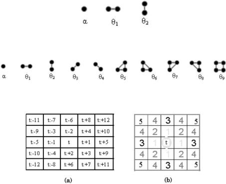
The structure of the neighborhood system determines the order of the MRF. For a first-order MRF the neighborhood of a pixel consists of its four nearest neighbors. In a second-order MRF the neighborhood consists of the eight nearest neighbors. The cliques structure are illustrated in Figs 9.1 and 9.2.

Consider a graph (t, η) as shown in Fig. 9.3 having a set of N2 sites. The energy function for a pairwise interaction model can be written in the following form: