

Kluwer - Handbook of Biomedical Image Analysis Vol
.1.pdf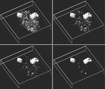
Co-Volume Level Set Method in Subjective Surface |
589 |
the presence of noise or in images with occlusions or subjective contours, these edges can be very irregular or even interrupted. Then the analysis of the scene and segmentation of objects become a difficult task.
In the so-called active contour models [32], an evolving family of curves converging to an edge is constructed. A simple approach (similar to various discrete region-growing algorithms) is to put small seed, e.g. small circular curve, inside the object and then evolve the curve to find automatically the object boundary. For such moving curves the level set models have been introduced in the last decade. A basic idea is that moving curve corresponds to a specific level line of the level set function which solves some reasonable generalization of Eq. (11.1). The level set methods have several advantages among which independence of dimension of the image and topology of objects are probably the most important. However, a reader can be interested also in the so-called direct (Lagrangian) approaches to curve and surface evolution (see e.g. [16–18, 39, 40]).
First simple level set model with the speed of segmentation curve modulated by g(| I0(x)|) (or more precisely by g(| Gσ I0|)), where g is a smooth edge detector function, e.g. g(s) = 1/(1 + K s2), has been given in [6] and [36]. In such a model, “steady state” of a particular level set (level line in 2D image) corresponds to boundary of a segmented object. Due to the shape of the Perona– Malik function g, the moving segmentation curve is strongly slowed down in a neighborhood of an edge, leading to a segmentation result. However, if an edge is crossed during evolution (which is not a rare event in noisy images), there is no mechanism to go back. Moreover, if there is a missing part of the object boundary, the algorithm is completely unuseful (as any other simple regiongrowing method).
Later on, the curve evolution and the level set models for segmentation have been significantly improved by finding a proper driving force in the form
− g(| I0(x)|) [7–9, 30, 31]. The vector field − g(| I0(x)|) has an important geometric property: It points toward regions where the norm of the gradient I0 is large (see Figs. 11.4 and 11.5). Thus if an initial curve belongs to a neighborhood of an edge, then it is driven toward this edge by this proper velocity field. Such motion can also be interpreted as a flow of the curve on surface g(| I0(x)|) subject to gravitational-like force driving the curve down to the narrow valley corresponding to the edge (see Fig. 11.6, [40]).
However, as one can see from Figs. 11.7 and 11.8, the situation is much more complicated in the case of noisy images. The advection process alone is


592 |
Mikula, Sarti, and Sgallari |
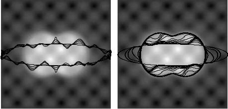
Figure 11.8: The evolution only by advection leads to attracting a curve (initial ellipse) to spurios edges, the evolution must be stopped without any reasonable segmentation result (left). By adding regularization term related to curvature of evolving curve, the edge is found smoothly (right).
curve evolution is given by Eq. (11.9), which is, of course, only another form of Eq. (11.8).
Although model (11.8) behaves very well if we are in the vicinity of an edge, it is sometimes difficult to drive the segmentation curve there. If we start with a small circular seed, it has large curvature and diffusion dominates advection so the seed disappears (curve shrinks to a point [22,23]). Then some constant speed must be added to dominate diffusion at the beginning of the process, but it is not clear at all when to switch off this driving force to have just the mechanism of the model (11.8). Moreover, in the case of missing boundaries of image objects, there is no criterion for such a switch, so the segmentation curve cannot be well localized to complete the missing boundaries.
An important observation now is that Eq. (11.8) moves not only one particular level line (segmentation curve) but all level lines by the above mentioned advection–diffusion mechanism. So, in spite of all previously mentioned segmentation approaches, we may start to think not on evolution of one particular level set but on evolution of the whole surface composed of those level sets. This idea to look on the solution u itself, i.e. on the behavior of our segmentation function, can help significantly.
Let us look on a simple numerical experiment presented in Fig. 11.10 representing extraction of the solid circle depicted in Fig. 11.9. The starting

Co-Volume Level Set Method in Subjective Surface |
593 |
|
|
|
|
|
|
|
Figure 11.9: Image of a solid circle.
point-of-view surface u0 is plotted on the top left. The subsequent evolution is depicted in the next subfigures. First, isolines which are close to the edge, i.e. in the neighborhood of the solid circle where the advection term is nonzero, are attracted from both sides to this edge. A small shock (steep gradient) is formed due to accumulation of these level lines (see Fig. 11.10 (top right)). In the regions outside the neighborhood of the circle, the advection term is vanishing and g0 ≡ 1, so only intrinsic diffusion of level sets plays a role. This means that all inside level sets are shrinking and finally they disappear. Such a process is nothing else but a decrease of the maximum of our segmentation function until the upper level of the shock is achieved. It is clear that a flat region in the profile of segmentation function inside the circle is formed. Outside of the circle, level sets are also shrinking until they are attracted by nonzero velocity field and then they contribute to the shock. In the bottom left of Fig. 11.10, we see the shape of segmentation function u after such evolution, in the bottom right there are isocontours of such function accumulated on the edges. It is very easy to use one of them, e.g., (max(u) + min(u))/2, to get the circle.
The situation is not so straightforward for the highly nonconvex image depicted in Fig. 11.11. Our numerical observation leads to formation of steps in subsequent evolution of the segmentation function, which is understandable, because very different level sets of initial surface u0 are attracted to different parts of the boundary of “batman.” Fortunately, we are a bit free in choosing the precise form of diffusion term in the segmentation model. After expansion of divergence, Eqs. (11.2) and (11.8) give the same advection term, g0 · u (cf. Eq. (11.9)), so important advection mechanism which accumulates segmentation function along the shock is the same. However, diffusion mechanisms are a

594 |
Mikula, Sarti, and Sgallari |
Figure 11.10: Subjective surface based segmentation of solid circle. We plot numerically computed time steps 0, 2, 10, 20, and 100. In the bottom right we see accumulation of level lines of segmentation function on the edges. In this experiment ε = 10−10, so we are very close to level set flow equation (11.8) (color slide).
bit different. Eq. (11.2), in the case ε = 1, gives diffusion which is known as mean curvature flow of graphs. It means that no level sets of segmentation function move in the normal direction proportionally to curvature, but the graph of segmentation function moves (as 2D surface in 3D space) in the normal direction proportionally to the mean curvature. The large variations in the graph of segmentation function are then smoothed due to large mean curvature. Of course,
Co-Volume Level Set Method in Subjective Surface |
595 |
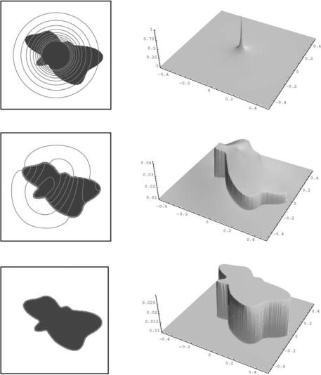
Figure 11.11: Subjective surface based segmentation of a “batman” image. In the left column we plot the black and white images to be segmented together with isolines of the segmentation function. In the right column there are shapes of the segmentation function. The rows correspond to time steps 0, 1, and 10, which gives the final result ε = 1 (color slide).
596 |
Mikula, Sarti, and Sgallari |
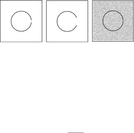
Figure 11.12: Three testing images. Circle with a smaller (left) and a big (middle) gap, and noisy circle with a gap.
the smoothing is applied only outside the edges. On the edges the advection dominates, since the mean curvature term is multiplied by a small value of g0. In Fig. 11.11 ( bottom) we may see formation of a piecewise flat profile of the segmentation function, which can be again very simply used for extraction of “batman,” although, due to Dirichlet boundary data and ε = 1, this profile moves slowly downwards in subsequent evolution. In this (academic) example, the only goal was to smooth (flatten) the segmentation function inside and outside the edge, so the choice ε = 1 was really satisfactory. In the case ε = 1, Eq. (11.2) can be interpreted as a time relaxation for the minimization of the weighted area functional
Ag0 = g0 1 + | u|2dx,
or as the mean curvature motion of a graph in Riemann space with metric g0δij
[48].
In the next three testing images plotted in Fig. 11.12 we illustrate the role of the regularization parameter ε. The same choice, ε = 1, as in the previous image with complete edge, is clearly not appropriate for image object with a gap (Fig. 11.12 (left)), as seen in Fig. 11.13. We see that minimal-surface-like diffusion closes the gap with a smoothly varying “waterfall” like shape. Although this shape is in a sense stable (it moves downwards in a “self-similar form”), it is not appropriate for segmentation purposes. However, decreasing ε, i.e., if we stay closer to the curvature-driven level set flow (11.8), or in other words, if we stretch the Riemannian metric g0δij in the vertical z direction [49], we get