Kluwer - Handbook of Biomedical Image Analysis Vol
.1.pdf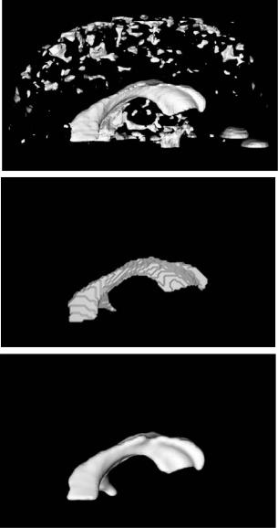
Level Set Segmentation of Biological Volume Datasets |
447 |
dataset (V2) is formed by calculating (C1, C2, C3) invariants for each voxel and combining them into Ca. It provides a measure of the magnitude of the anisotropy within the volume. Higher values identify regions of greater spatial anisotropy in the diffusion properties. A slice from the second scalar volume is presented in Fig. 8.12 (right). The measure Ca does not by definition distinguish between linear and planar anisotropy. This is sufficient for our current study since the brain does not contain measurable regions with planar diffusion anisotropy. We therefore only need two scalar volumes in order to segment the DT dataset.
We then utilize our level set framework to extract smoothed models from the two derived scalar volumes. First the input data is filtered with a low-pass Gaussian filter (σ ≈ 0.5) to blur the data and thereby reduce noise. Next, the volume voxels are classified for inclusion/exclusion in the initialization based on the filtered values of the input data (k ≈ 7.0 for V1 and k ≈ 1.3 for V2). For grayscale images, such as those used in this chapter, the classification is equivalent to high and low thresholding operations. The last initialization step consists of performing a set of topological (e.g. flood fill) operations in order to remove small pieces or holes from objects. This is followed by a level set deformation that pulls the surface toward local maxima of the gradient magnitude and smooths it with a curvature-based motion. This moves the surface toward specific features in the data, while minimizing the influence of noise in the data.
Figures 8.13 and 8.14 present two models that we extracted from DT-MRI volume datasets using our techniques. Figure 8.13 contains segmentations from volume V1, the measure of total diffusivity. The top image shows a Marching Cubes isosurface using an isovalue of 7.5. In the bottom we have extracted just the ventricles from V1. This is accomplished by creating an initial model with a flood-fill operation inside the ventricle structure shown in the middle image. This identified the connected voxels with value of 7.0 or greater. The initial model was then refined and smoothed with a level set deformation, using a β value of 0.2.
Figure 8.14 again provides the comparison between direct isosurfacing and and level set modeling, but on the volume V2. The image in the top-left corner is a Marching Cubes isosurface using an isovalue of 1.3. There is significant highfrequency noise and features in this dataset. The challenge here was to isolate coherent regions of high anisotropic diffusion. We applied our segmentation approach to the dataset and worked with neuroscientists from LA Childrens

448 |
|
Breen, Whitaker, Museth, and Zhukov |
|
|
|
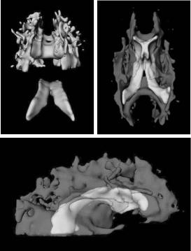
Figure 8.14: Model segmentation from volume V2. Top left image is an isosurface of value 1.3, used for initialization of the level set. Clockwise are the results of level set development with corresponding β values of 0.2, 0.4, and 0.5.
Hospital, City of Hope Hospital and Caltech to identify meaningful anatomical structures. We applied our approach using a variety of parameter values, and presented our results to them, asking them to pick the model that they felt best represented the structures of the brain. Figure 8.14 contains three models extracted from V2 at different values of smoothing parameter β used during segmentation. Since we were not looking for a single connected structure in this volume, we did not use a seeded flood-fill for initialization. Instead, we initialized the deformation process with an isosurface of value 1.3. This was followed by a level set deformation using a β value of 0.2. The result of this segmentation is presented on the bottom-left side of Fig. 8.14. The top-right side of this figure presents a model extracted from V2 using an initial isosurface of value 1.4 and a
β value of 0.5. The result chosen as the “best” by our scientific/medical collaborators is presented on the bottom-right side of Fig. 8.14. This model is produced with an initial isosurface of 1.3 and a β value of 0.4. Our collaborators were able to identify structures of high diffusivity in this model, for example the corpus callosum, the internal capsul, the optical nerve tracks, and other white matter regions.
Level Set Segmentation of Biological Volume Datasets |
449 |
Figure 8.15: Combined model of ventricles and (semi-transparent) anisotropic regions: rear, exploded view (left), bottom view (right), side view (bottom). Note how model of ventricles extracted from isotropic measure dataset V1 fits into model extracted from anisotropic measure dataset V2.
We can also bring together the two models extracted from datasets V1 and V2 into a single image. They will have perfect alignment since they are derived from the same DT-MRI dataset. Figure 8.15 demonstrates that we are able to isolate different structures in the brain from a single DT-MRI scan and show their proper spatial interrelationship. For example, it can be seen that the corpus callosum lies directly on top of the ventricles, and that the white matter fans out from both sides of the ventricles.
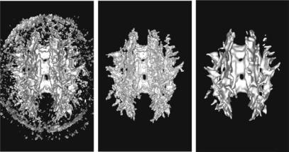
Finally, to verify the validity of our approach we applied it to the second dataset from a different volunteer. This dataset has 20 slices of the 256 × 256 resolution. We generated the anisotropy measure volume V2 and performed the level set model extraction using the same isovalues and smoothing parameters as for V2. The results are shown in Fig. 8.16, and demonstrate the generality of our approach.
450 |
Breen, Whitaker, Museth, and Zhukov |
Figure 8.16: Segmentation using anisotropic measure V2 from the second DTMRI dataset. (left) Marching Cubes isosurface with iso-value 1.3. (middle) Result of flood-fill algorithm applied to the volume and used for initialization. (right) Final level set model.
8.6Direct Estimation of Surfaces in Tomographic Data
The radon transform is invertible (albeit, marginally so) when the measured data consists of a sufficient number of good quality, properly spaced projections [73]. However, for many applications the number of realizable projections is insufficient, and direct grayscale reconstructions are susceptible to artifacts. We will refer to such problems as underconstrained tomographic problems. Cases of underconstrained tomographic problems usually fall into one of two classes. The first class is where the measuring device produces a relatively dense set of projections (i.e. adequately spaced) that do not span a full 180◦. In these cases, the sinogram contains regions without measured data. Considering the radon transform in the Fourier domain, these missing regions of the sinogram correspond to a transform with angular wedges (pie slices) that are null, making the transform noninvertible. We assume that these missing regions are large enough to preclude any straightforward interpolation in the frequency domain. The second class of incomplete tomographic problems are those that consist of an insufficient number of widely spaced projections. We assume that these sparse samples of the sinogram space are well distributed over a wide range of angles. For this discussion the precise spacing is not important. This problem
Level Set Segmentation of Biological Volume Datasets |
451 |
is characterized by very little data in the Fourier domain, and direct inversion approaches produce severe artifacts. Difficulties in reconstructing volumes from such incomplete tomographic datasets are often aggravated by noise in the measurements and misalignments among projections.
Under-constrained problems are typically solved using one or both of two different strategies. The first strategy is to choose from among feasible solutions (those that match the data) by imposing some additional criterion, such as finding the solution that minimizes an energy function. This additional criterion should be designed to capture some desirable property, such as minimum entropy. The second strategy is to parameterize the solution in a way that reduces the number of degrees of freedom. Normally, the model should contain few enough parameters so that the resulting parameter estimation problem is overconstrained. In such situations solutions are allowed to differ from the data in a way that accounts for noise in the measurements.
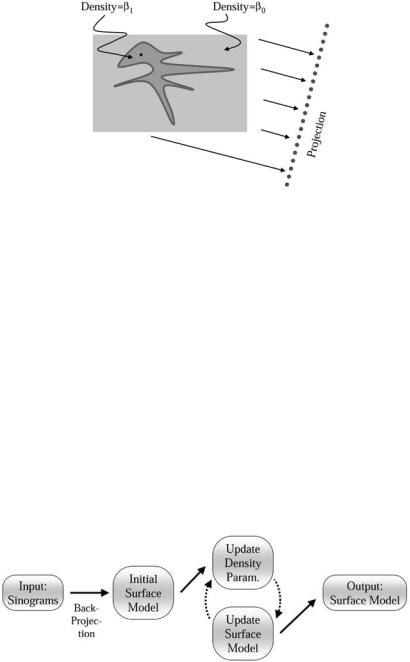
In this section we consider a special class of underconstrained tomographic problems that permits the use of a simplifying model. The class of problems we consider are those in which the imaging process is targeted toward tissues or organs that have been set apart from the other anatomy by some contrast agent. This agent could be an opaque dye, as in the case of transmission tomography, or an emissive metabolite, as in nuclear medicine. We assume that this agent produces relatively homogeneous patches that are bounded by areas of high contrast. This assumption is reasonable, for instance, in subtractive angiography or CT studies of the colon. The proposed approach, therefore, seeks to find the boundaries of different regions in a volume by estimating sets of closed surface models and their associated density parameters directly from the incomplete sinogram data [74]. Thus, the reconstruction problem is converted to a segmentation problem. Of course, we can never expect real tissues to exhibit truly homogeneous densities. However, we assert that when inhomogeneities are somewhat uncorrelated and of low contrast the proposed model is adequate to obtain acceptable reconstructions.
8.6.1 Related Work
Several areas of distinct areas of research in medical imaging, computer vision, and inverse problems impact this work. Numerous tomographic reconstruction methods are described in the literature [75, 76], and the method of choice depends on the quality of projection data. Filtered back projection (FBP), the
Level Set Segmentation of Biological Volume Datasets |
453 |
density β0 and collection of solid objects with density β1. We denote the (open) set of points in those regions as , the closure of that set, the surface, as S.
The projection of a 2D signal f (x, y) produces a sinogram given by the radon transform as
+∞ |
+∞ |
|
|
p(s, θ ) = −∞ |
−∞ |
f (x, y)δ(Rθ x − s)dx, |
(8.33) |
where Rθ x = x cos(θ ) + y sin(θ ) is a rotation and projection of a point x = (x, y) onto the imaging plane associated with θ . The 3D formulation is the same, except that the signal f (x, y, z) produces a collection of images. We denote the projection of the model, which includes estimates of the objects and the background, as
p(s, θ ). For this work we denote the angles associated with a discrete set of projections as θ1, . . . , θN and denote the domain of each projection as S = s1, . . . sM . Our strategy is to find , β0, and β1 by maximizing the likelihood.
If we assume the projection measurements are corrupted by independent noise, the log likelihood of a collection of measurements for a specific shape and density estimate is the probability of those measurements conditional on the model,
ln P( p(s1, θ1), p(s2, θ1), . . . , p(sM , θN )|S, β0, β1)
=ln P( p(sj , θi)|S, β0, β1). (8.34)
i j
We call the negative log likelihood the error and denote it Edata. Normally, the probability density of a measurement is parameterized by the ideal value, which gives
|
|
|
|
|
N |
M |
|
|
|
Edata = |
j=1 |
E pij , pij , |
(8.35) |
|
i=1 |
|
|
|
|
where E( pi, j , pi, j ) = − ln P( pi, j , pi, j ) is the error associated with a particular point in the radon space, and pi, j = p(sj , θi). In the case of independent Gaussian noise, E is a quadratic, and the log likelihood results in a weighted least-squares in the radon space. For all of our results, we use a Gaussian noise model. Next we apply the object model, shown in Fig. 8.17, to the reconstruction of f . If we let g(x, y) be a binary inside–outside function on , then we have the following approximation to f (x, y):
f (x, y) ≈ β0 + [β1 − β0]g(x, y). |
(8.36) |