

Kluwer - Handbook of Biomedical Image Analysis Vol
.1.pdfWavelets in Medical Image Processing |
335 |
Because the wavelet basis ψ 1, ψ 2, and ψ 3 are first derivatives of a cubic spline function θ , the three components of a wavelet coefficient Wmk s(n1, n2, n3) =, k = 1, 2, 3, are proportional to the coordinates of the gradient vector of the input image s smoothed by a dilated version of θ . From these coor-
dinates, one can compute the angle of the gradient vector, which indicates the direction in which the first derivative of the smoothed s has the largest amplitude (or the direction in which s changes most rapidly). The amplitude of this maximized first derivative is equal to the modulus of the gradient vector, and
therefore proportional to the wavelet modulus: |
|
|
|
|
|
||||||
Mms = |
|
|
|
|
|
|
. |
(6.44) |
|||
Wm1 s 2 |
+ |
Wm2 s 2 |
+ |
Wm3 s 2 |
|||||||
|
|
|
|
|
|
|
|
|
|
|
|
Thresholding this modulus value instead of the coefficient value consists of first selecting a direction in which the partial derivative is maximum at each scale, and then thresholding the amplitude of the partial derivative in this direction. The modified wavelet coefficients are then computed from the thresholded modulus and the angle of the gradient vector. Such paradigm applies an adaptive choice of the spatial orientation in order to best correlate the signal features with the wavelet coefficients. It can therefore provide a more robust and accurate selection of correlated signals compared to traditional orientation selection along three orthogonal Cartesian directions.
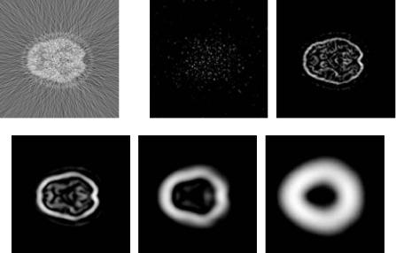
Figure 6.20 illustrates the performance of this approach at denoising a clinical brain PET data set reconstructed by FBP with a ramp filter. The reconstructed PET images, illustrated for one slice in Fig. 6.20(a), contain prominent noise in high frequency but do not express strong edge features in the wavelet modulus expansions at scale 1 through 5 as illustrated in Fig. 6.20(b)–(f).
Cross-Scale Regularization for Images with Low SNR. As shown in Fig. 6.20(b), very often in tomographic images, the first level of expansion (level with more detailed information) is overwhelmed by noise in a random pattern. Thresholding operators determined only by the information in this multiscale level can hardly recover useful signal features from the noisy observation. On the other hand, wavelet coefficients in the first level contain the most detailed information in a spatial-frequency expansion, and therefore influence directly the spatial resolution of the reconstructed image.
To have more signal-related coefficients recovered, additional information or a priori knowledge is needed. Intuitively, an edge indication map could
336 |
Jin, Angelini, and Laine |
(a) |
(b) |
(c) |
(d) |
(e) |
(f ) |
Figure 6.20: (a) A brain PET image from a 3D data set with high level of noise.
(b)–(f) Modulus of wavelet coefficients at expansion scale 1 to 5.
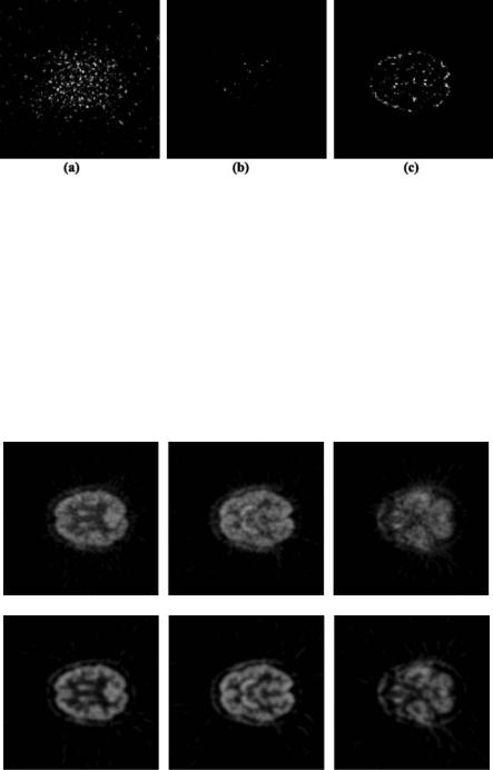
beneficially assist such wavelet expansion based on first derivative of spline wavelets. Without seeking external a priori information, it was observed that wavelet modulus from the next higher wavelet level can serve as a good edge estimation. An edge indication map with values between 0 and 1 (analogous to the probability that a pixel is located on an edge) was therefore constructed by normalizing the modulus of this subband. A pixel-wise multiplication of the edge indication map and the first level wavelet modulus can identify the location of wavelet coefficients that are more likely to belong to a true anatomical edge and should be preserved, as well as the locations of the wavelet coefficients that are unlikely to be related to real edge signal and that should be attenuated. This approach is referred to as cross-scale regularization. A comparison between traditional wavelet shrinkage and cross-scale regularization for recovering useful signals from the most detailed level of wavelet modulus is provided in Fig. 6.21.
A cross-scale regularization process does not introduce any additional parameter avoiding extra complexity for algorithm optimization and automation. We point out that an improved edge indication prior can be built upon a modified wavelet modulus in the next spatial-frequency scale processed using traditional thresholding and enhancement operator.
Wavelets in Medical Image Processing |
337 |
Figure 6.21: (a) Wavelet modulus in first level of a PET brain image as shown in Figs. 6.20 (a) and (b). (b) Thresholding of the wavelet modulus from (a) using a wavelet shrinkage operator. (c) Thresholding of the wavelet modulus from (a) with cross-scale regularization.
Spatial-frequency representations of a signal after wavelet expansion offer the possibility to adaptively process an image data in different sub-bands. Such adaptive scheme can for example combine enhancement of wavelet coefficients in the coarse levels, and resetting of the most detailed levels for noise suppression. We show in Fig. 6.22 how such adaptive processing can remarkably
FBP Reconstruction (Hann windows)
Adaptive Multiscale Denoising and Enhancement
Figure 6.22: Denoising of PET brain data and comparison between unprocessed and multiscale processed images.
338 |
Jin, Angelini, and Laine |
improve image quality for PET images that were usually degraded by low resolution and high level of noise.
6.4 Image Segmentation Using Wavelets
6.4.1Multiscale Texture Classification and Segmentation
Texture is an important characteristic for analyzing many types of images, including natural scenes and medical images. With the unique property of spatialfrequency localization, wavelet functions provide an ideal representation for texture analysis. Experimental evidence on human and mammalian vision support the notion of spatial-frequency analysis that maximizes a simultaneous localization of energy in both spatial and frequency domains [69–71]. These psychophysical and physiological findings lead to several research works on texture-based segmentation methods based on multiscale analysis.
Gabor transform, as suggested by the uncertainty principle, provides an optimal joint resolution in the space-frequency domain. Many early works utilized Gabor transforms for texture characteristics. In [27] an example is given on the use of Gabor coefficient spectral signatures [72] to separate distinct textural regions characterized by different orientations and predominant anisotropic texture moments. Porat et al. proposed in [28] six features derived from Gabor coefficients to characterize a local texture component in an image: the dominant localized frequency; the second moment (variance) of the localized frequency; center of gravity; variance of local orientation; local mean intensity; and variance of the intensity level. A simple minimum-distance classifier was used to classify individual textured regions within a single image using these features.
Many wavelet-based texture segmentation methods had been investigated thereafter. Most of these methods follow a three-step procedure: multiscale expansion, feature characterization, and classification. As such, they are usually different from each other in these aspects.
Various multiscale representations have been used for texture analysis. Unser [73] used a redundant wavelet frame. Laine et al. [74] investigated a wavelet packets representation and extended their research to a redundant wavelet packets frame with Lemarie´–Battle filters in [75]. Modulated wavelets
Wavelets in Medical Image Processing |
339 |
were used in [76] for better orientation adaptivity. To further extend the flexibility of the spatial-frequency analysis, a multiwavelet packet, combining multiple wavelet basis functions at different expansion levels, was used in [77]. An M- band wavelet expansion, which differs from a dyadic wavelet transform in the fact that each expansion level contains M channels of analysis, was used in [78] to improve orientation selectivity.
Quality and accuracy of segmentation ultimately depend on the selection of the characterizing features. A simple feature selection can use the amplitude of the wavelet coefficients [76]. Many multiscale texture segmentation methods construct the feature vector from various local statistics of the wavelet coefficients, such as its local variance [73, 79], moments [80], or energy signature [74, 78, 81]. Wavelet extrema density, defined as the number of extrema of wavelet coefficients per unit area, was used in [77]. In [75], a 1D envelope detection was first applied to the wavelet packets coefficients according to their orientation, and a feature vector was constructed as the collection of envelope values for each spatial-frequency component. More sophisticated statistical analyses involving Bayesian analysis and Markov random fields (MRF) were also used to estimate local and long-range correlations [82, 83]. Other multiscale textural features were also reported, for example χ 2 test and histogram testing were used in [84], “Roughness” based on fractal dimension measurement was used in [85].
Texture-based segmentation is usually achieved by texture classification. Classic classifiers, such as the minimum distance classifier [28], are easier to implement when the dimension of the feature vector is small and the groups of samples are well segregated. The most popular classification procedures reported in the literature are the K-mean classifier [73, 75, 76, 78, 79, 81, 85] and the neural networks classifiers [27, 74, 80, 82].
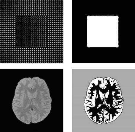
As an example, we illustrate in Fig. 6.23 a texture-based segmentation method on a synthetic texture image and a medical image from a brain MRI data set. The algorithm used for this example from [75] uses the combination of wavelet packets frame with Lemarie´–Battle filters, multiscale envelope features, and a
K-mean classifier.
6.4.2 Wavelet Edge Detection and Segmentation
Edge detection plays an important role in image segmentation. In many cases, boundary delineation is the ultimate goal for an image segmentation and a good
340 |
Jin, Angelini, and Laine |
(a) |
(b) |
(c) |
(d) |
Figure 6.23: Sample results using multiscale texture segmentation. (a) Synthetic texture image. (b) Segmentation result for image (a) with a 2-class labeling. (c) MRI T1 image of a human brain. (d) Segmentation result for image (c) with a 4-class labeling.
edge detector itself can then fulfill the requirement of segmentation. On the other hand, many segmentation techniques require an estimation of object edges for their initialization. For example, with standard gradient-based deformable models, an edge map is used to determine where the deforming interface must stop. In this case, the final result of the segmentation method depends heavily on the accuracy and completeness of the initial edge map. Although many research works have made some efforts to eliminate this type of interdependency by
Wavelets in Medical Image Processing |
341 |
introducing nonedge constraints [86, 87], it is necessary and equally important to improve the edge estimation process itself.
As pointed out by the pioneering work of Mallat et al. [16], firstor second- derivative-based wavelet functions can be used for multiscale edge detection. Most multiscale edge detectors smooth the input signal at various scales and detect sharp variation locations (edges) from their first or second derivatives. Edge locations are related to the extrema of the first derivative of the signal and the zero crossings of the second derivative of the signal. In [16], it was also pointed out that first-derivative wavelet functions are more appropriate for edge detection since the magnitude of wavelet modulus represents the relative “strength” of the edges, and therefore enable to differentiate meaningful edges from small fluctuations caused by noise.
Using the first derivative of a smooth function θ (x, y) as the mother wavelet of a multiscale expansion results in a representation where the two components of wavelet coefficients at a certain scale s are related to the gradient vector of the input image f (x, y) smoothed by a dilated version of θ (x, y) at scale s:
|
1 |
f (x, y) |
|
|
Ws |
|
|
||
W |
2 |
f (x, y) |
= s ( f θs)(x, y). |
(6.45) |
|
s |
|
|
|
The direction of the gradient vector at a point (x, y) indicates the direction in the image plane along which the directional derivative of f (x, y) has the largest absolute value. Edge points (local maxima) can be detected as points (x0, y0) such that the modulus of the gradient vector is maximum in the direction toward which the gradient vector points in the image plane. Such computation is closely related to a Canny edge detector [88]. Extension to higher dimension is quite straightforward.
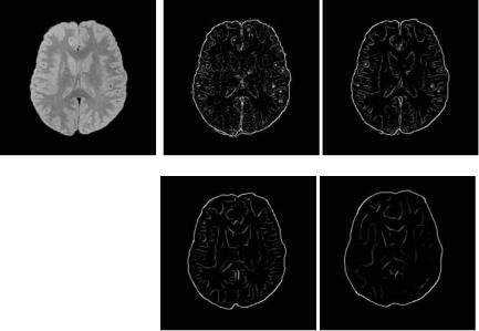
Figure 6.24 provides an example of a multiscale edge detection method based on a first derivative wavelet function.
To further improve the robustness of such a multiscale edge detector, Mallat and Zhong [16] also investigated the relations between singularity (Lipschitz regularity) and the propagation of multiscale edges across wavelet scales. In [89], the dyadic expansion was extended to an M-band expansion to increase directional selectivity. Also, continuous scale representation was used for better adaptation to object sizes [90]. Continuity constraints were applied to fully recover a reliable boundary delineation from 2D and 3D cardiac ultrasound in [91]
342 |
Jin, Angelini, and Laine |
(a) |
(b) |
(c) |
(d) |
(e) |
Figure 6.24: Example of a multiscale edge detection method finding local maxima of wavelet modulus, with a first-derivative wavelet function. (a) Input image and (b)–(e) multiscale edge map at expansion scale 1 to 4.
and [92]. In [93], both cross-scale edge correlations and spatial continuity were investigated to improve the edge detection in the presence of noise. Wilson et al. in [94] also suggested that a multiresolution Markov model can be used to track boundary curves of objects from a multiscale expansion using a generalized wavelet transform.
Given their robustness and natural representation as boundary information within a multiresolution representation, multiscale edges have been used in deformable model methods to provide a more reliable constraint on the model deformation {Yoshida, 1997 #3686; de Rivaz, 2000 #3687; Wu, 2000 #3688; Sun, 2003 #3689}, as an alternative to traditional gradient-based edge map. In [99], it was used as a presegmentation step in order to find the markers that are used by watershed transform.
6.4.3 Other Wavelet-Based Segmentation
One important feature of wavelet transform is its ability to provide a representation of the image data in a multiresolution fashion. Such hierarchical
Wavelets in Medical Image Processing |
343 |
decomposition of the image information provides the possibility of analyzing the coarse resolution first, and then sequentially refines the segmentation result at more detailed scales. In general, such practice provides additional robustness to noise and local maxima.
In [100], image data was first decomposed into “channels” for a selected set of resolution levels using a wavelet packets transform. An MRF segmentation was then applied to the subbands coefficients for each scale, starting with the coarsest level and propagating the segmentation result from one level to initialize the segmentation at the next level.
More recently, Davatzikos et al. [101] proposed hierarchical active shape models where the statistical properties of the wavelet transform of a deformable contour were analyzed via principal component analysis and used as priors for constraining the contour deformations.
Many research works beneficially used image features within a spatialfrequency domain after wavelet transform to assist the segmentation. In [102] Strickland et al. used image features extracted in the wavelet transform domain for detection of microcalcifications in mammograms using a matching process and a priori knowledge on the target objects (microcalcification). In [103], Zhang et al. used a Bayes classifier on wavelet coefficients to determine an appropriate scale and threshold that can separate segmentation targets from other features.
6.5 Image Registration Using Wavelets
In this section, we give a brief overview of another very important application of wavelets in image processing: image registration. Readers interested in this topic are encouraged to read the references listed in the context.
Image registration is required for many image processing applications. In medical imaging, co-registration problems are important for many clinical tasks:
1.multimodalities study,
2.cross-subject normalization and template/atlas analysis,
3.patient monitoring over time with tracking of the pathological evolution for the same patient and the same modality.
344 |
Jin, Angelini, and Laine |
Many registration methods follow a feature matching procedure. Feature points (often referred to as “control points,” or CP) are first identified in both the reference image and the input image. An optimal spatial transformation (rigid or nonrigid) is then computed that can connect and correlate the two sets of control points with minimal error. Registration has always been considered as very costly in terms of computational load. Besides, when the input image is highly deviated from the reference image, the optimization process can be easily trapped into local minima before reaching the correct transformation mapping. Both issues can be alleviated by embedding the registration into a “coarse to fine” procedure. In this framework, the initial registration is carried out on a relatively low resolution image data, and sequentially refined to higher resolution. Registration at higher resolution is initialized with the result from the lower resolution and only needs to refine the mapping between the two images with local deformations for updating the transformation parameters.
The powerful representation provided by the multiresolution analysis framework with wavelet functions has lead many researchers to use a wavelet expansion for such “coarse to fine” procedures [104–106]. As already discussed previously, the information representation in the wavelet transform domain offers a better characterization of key spatial features and signal variations. In addition to a natural framework for “coarse to fine” procedure, many research works also reported the advantages of using wavelet subbands for feature characterization. For example, in [107] Zheng et al. constructed a set of feature points from a Gabor wavelet model that represented local curvature discontinuities. They further required that a feature point should have maximum energy among a neighborhood and above a certain threshold. In [108], Moigne et al. used wavelet coefficients with magnitude above 13–15% of the maximum value to form their feature space. In [109], Dinov et al. applied a frequency adaptive thresholding (shrinkage) to the wavelet coefficients to keep only significant coefficients in the wavelet transform domain for registration.
6.6 Summary
This chapter provided an introduction to the fundamentals of multiscale transform theory using wavelet functions. The versatility of these multiscale