Kluwer - Handbook of Biomedical Image Analysis Vol

overviews the theoretical fundamentals of wavelet theory and related multiscale representations. As an example, the implementation of an overcomplete dyadic wavelet transform will be illustrated. Section 6.3 includes a general introduction of image denoising and enhancement techniques using wavelet analysis. Sections 6.4 and 6.5 summarize the basic principles and research works in literature for wavelet analysis applied to image segmentation and registration.

6.2Wavelet Transform and Multiscale Analysis

One of the most fundamental problems in signal processing is to find a suitable representation of the data that will facilitate an analysis procedure. One way to achieve this goal is to use transformation, or decomposition of the signal on a set of basis functions prior to processing in the transform domain. Transform theory has played a key role in image processing for a number of years, and it continues to be a topic of interest in theoretical as well as applied work in this field. Image transforms are used widely in many image processing fields, including image enhancement, restoration, encoding, and description [12].

Historically, the Fourier transform has dominated linear time-invariant signal processing. The associated basis functions are complex sinusoidal waves eiωt that correspond to the eigenvectors of a linear time-invariant operator. A signal f (t) defined in the temporal domain and its Fourier transform fˆ(ω), defined in

the frequency domain, have the following relationships [12, 13]:

Fourier transform characterizes a signal f (t) via its frequency components. Since the support of the bases function eiωt covers the whole temporal domain (i.e. infinite support), fˆ(ω) depends on the values of f (t) for all times. This makes the Fourier transform a global transform that cannot analyze local or transient properties of the original signal f (t).

In order to capture frequency evolution of a nonstatic signal, the basis functions should have compact support in both time and frequency domains. To achieve this goal, a windowed Fourier transform (WFT) was first introduced

The low-frequency approximation of a signal f at the scale s is computed as:

For a one-dimensional signal f , the continuous wavelet transform (6.7) is a twodimensional representation. This indicates the existence of redundancy that can be reduced and even removed by subsampling the scale parameter s and translation parameter u.

An orthogonal (nonredundant) wavelet transform can be constructed constraining the dilation parameter to be discretized on an exponential sampling with fixed dilation steps and the translation parameter by integer multiples of a dilation-dependent step [15]. In practice, it is convenient to follow a dyadic scale sampling where s = 2i and u = 2i · k, with i and k being integers. With dyadic

dilation and scaling, the wavelet basis function, defined as:

forms an orthogonal basis of L2(R).

For practical purpose, when using orthogonal basis functions, the wavelet transform defined in Eq. (6.7) is only computed for a finite number of scales (2J ) with {J = 0, . . . , N}, and a low-frequency component L f (u, 2J ) (often referred to as the DC component) is added to the set of projection coefficients corresponding to scales larger than 2J for a complete signal representation.

In medical image processing applications, we usually deal with discrete data. We will therefore focus the rest of our discussion on discrete wavelet transform rather than continuous ones.

6.2.2 Discrete Wavelet Transform and Filter Bank

Given a 1D signal of length N, { f (n), n = 0, . . . , N − 1}, the discrete orthogonal wavelet transform can be organized as a sequence of discrete functions according to the scale parameter s = 2 j :

where L J f = L f (2J n, 2J ) and W j f = W f (2 j n, 2 j ).

h[-n] ↓ 2 L2 f

h[-n] ↓ 2 L1 f

g[-n] ↓ 2 W1 f

↓ 2 downsampling by 2

Figure 6.2: Illustration of orthogonal wavelet transform of a discrete signal f (n) with CMF. A two-level expansion is shown.

Wavelet coefficients W j f at scale s = 2 j have a length of N/2 j and the largest decomposition depth J is bounded by the signal length N as (sup( J) = log2 N).

For fast implementation (such as filter bank algorithms), a pair of conjugate mirror filters (CMF) h and g can be constructed from the scaling function φ and

It can be proven that h is a low-pass filter and g is a high-pass filter. The discrete orthogonal wavelet decomposition in Eq. (6.11) can be computed by applying these two filters to the input signal and recursively decomposing the low-pass band, as illustrated in Fig. 6.2. A detailed proof can be found in [15].

For orthogonal basis, the input signal can be reconstructed from wavelet coefficients computed in Eq. (6.11) using the same pair of filters, as illustrated in Fig. 6.3.

↑ 2 upsampling by 2

Figure 6.3: Illustration of inverse wavelet transform implemented with CMF. A

two-level expansion is shown.

It is easy to prove that the total amount of data after a discrete wavelet expansion as shown in Fig. 6.2 has the same length to the input signal. Therefore, such transform provides a compact representation of the signal suited to data compression as wavelet transform provides a better spatial-frequency localization. On the other hand, since the data was downsampled at each level of expansion, such transform performs poorly on localization or detection problems. Mathematically, the transform is variant under translation of the signal (i.e. is dependent on the downsampling scheme used during the decomposition), which makes it less attractive for analysis of nonstationary signals. In image analysis, translation invariance is critical to the preservation of all the information of the signal and a redundant representation needs to be applied.

In the dyadic wavelet transform framework proposed by Mallat et al. [16], sampling of the translation parameter was performed with the same sampling period as that of the input signal in order to preserve translation invariance.

A more general framework of wavelet transform can be designed with different reconstruction and decomposition filters that form a biorthogonal basis. Such generalization provides more flexibility in the design of the wavelet functions. In that case, similar to Eq. (6.11), the discrete dyadic wavelet transform of a signal s(n) is defined as a sequence of discrete functions:

where SM s(n) = s φM (n) represents the DC component, or the coarsest information from the input signal.

Given a pair of wavelet function ψ (x) and reconstruction function χ (x), the discrete dyadic wavelet transform (decomposition and reconstruction) can be implemented with a fast filter bank scheme using a pair of decomposition filters

H, G and a reconstruction filter K [16]:

Defining Fs(ω) = e−iωs F(ω), where F is H, G, or K , we can construct a filter bank implementation of the discrete dyadic wavelet transform as illustrated in

Figure 6.4: Filter bank implementation of a one-dimensional discrete dyadic wavelet transform decomposition and reconstruction for three levels of analysis.

Hs (ω) denotes the complex conjugate of Hs(ω).

Fig. 6.4. Filters F(2m ω) defined at level m + 1 (i.e., filters applied at wavelet scale 2m) are constructed by inserting 2m − 1 zeros between subsequent filter coefficients from level 1 (F(ω)). Noninteger shifts at level 1 are rounded to the nearest integer. This implementation design is called “algorithme a` trous” [17, 18] and has a complexity that increases linearly with the number of analysis levels.

In image processing applications, we often deal with two, three, or even higher dimensional data. Extension of the framework to higher dimension is quite straightforward. Multidimensional wavelet bases can be constructed with tensor products of separable basis functions defined along each dimension. In that context, an N-dimensional discrete dyadic wavelet transform with M

where Wmk s = s, ψmk represents the detailed information along the kth coordinate at scale m. The wavelet basis is dilated and translated from a set of separable wavelet functions ψ k, k = 1, . . . , N, for example in 3D:

(6.18)

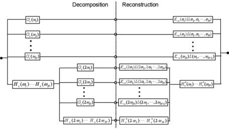
Figure 6.5: Filter bank implementation of a multidimensional discrete dyadic wavelet transform decomposition (left) and reconstruction (right) for two levels of analysis.

In this framework, reconstruction with an N-dimensional dyadic wavelet transform requires a nonseparable filter L N to compensate the interdimension correlations. This is formulated in a general context as:

Figure 6.5 illustrates a filter bank implementation with a multidimensional discrete dyadic wavelet transform. For more details and discussions we refer to [19].

6.2.3 Other Multiscale Representations

Wavelet transforms are part of a general framework of multiscale analysis. Various multiscale representations have been derived from the spatial-frequency framework offered by wavelet expansion, many of which were introduced to provide more flexibility for the spatial-frequency selectivity or better adaptation to real-world applications.

In this section, we briefly review several multiscale representations derived from wavelet transforms. Readers with an intention to investigate more

theoretical and technical details are referred to the textbooks on Gabor analysis [20], wavelet packets [21], and the original paper on brushlet [22].

6.2.3.1 Gabor Transform and Gabor Wavelets

In his early work, Gabor [23] suggested an expansion of a signal s(t) in terms of time–frequency atoms gm,n(t) defined as:

where gm,n(t), m, n Z, are constructed with a window function g(x), combined to a complex exponential:

Gabor also suggested that an appropriate choice for the window function g(x) is the Gaussian function due to the fact that a Gaussian function has the theoretically best joint spatial-frequency resolution (uncertainty principle). It is important to note here that the Gabor elementary functions gm,n(t) are not orthogonal and therefore require a biorthogonal dual function γ (x) for reconstruction [24]. This dual window function is used for the computation of the expansion coefficients cm,n as:

while the Gaussian window is used for the reconstruction.

The biorthogonality of the two window functions γ (x) and g(x) is expressed

as:

From Eq. (6.21), it is easy to see that all spatial-frequency atom gm,n(t) share the same spatial-frequency resolution defined by the Gaussian function g(x). As pointed out in the discussion on short-time Fourier transforms, such design is suboptimal for the analysis of signals with different frequency components.

A wavelet-type generalization of Gabor expansion can be constructed such that different window functions are used instead of a single one [25] according to their spatial-frequency location. Following the design of wavelets, a Gabor