

Kluwer - Handbook of Biomedical Image Analysis Vol
.1.pdfLevel Set Segmentation of Biological Volume Datasets |
|
|
|
|
455 |
|||||||
sinogram data. The incremental change in the likelihood is |
|
|
|
|||||||||
|
|
|
|
|
|
|
|
(8.38) |
||||
|
dEdata |
N |
M |
d |
|
|
N |
M |
|
|
d pij |
|
|
dt |
= S i=1 j=1 |
dt |
E pij , pi, j dx = |
S i=1 j=1 E pij , pij |
|
dt |
dx, |
||||
where E = ∂ E/∂ p, which, for Gaussian noise, is simply the difference between
|
. |
must formulate |
d p/dt |
, which, by the transport equation, is |
||||||||
p and p Next we |
|
|
|
|
|
|
|
|
||||
|
|
|
|
|
|
|
d |
|
|
|
|
|
|
d pij |
|
[β1 |
|
β0] |
δ(Rθ x |
|
sj )dx |
|
|||
|
|
dt |
= |
|
− |
|
dt |
|
i |
− |
|
|
|
|
|
= [β1 |
− β0] |
S δ(Rθi x − sj )n(x) · v(x)dx, |
(8.39) |
||||||
where n is an outward pointing surface normal and v(x) is the velocity of the surface at the point x. The derivative of Edata with respect to surface motion is therefore
|
|
|
|
|
|
dEdata |
N |
M |
|
|
|
dt |
= [β1 − β0] S i=1 |
j=1 |
E |
pi, j , pij δ(Rθi x − sj )n(x) · v(x) dx. (8.40) |
|
Note that the integral over dx and the δ functional serve merely to associate sj in the ith scan with the appropriate x point. If the samples in each projection are sufficiently dense, we can approximate the sum over j as an integral over the image domain, and thus for every x on the surface there is a mapping back into the ith projection. We denote this point si(x). This gives a closed-form expression for the derivative of the derivative of Edata in terms of the surface velocity,
|
|
|
|
dEdata |
N |
|
|
dt |
= [β1 − β0] S i=1 |
ei(x)n(x) · v(x)dx, |
(8.41) |
where ei(x) = E ( p(si(x), θi), p(si(x), θi)) is the derivative of the error associated with the point si(x) in the ith projection. The result shown in Eq. (8.41) does not make any specific assumptions about the surface shape or its representation. Thus, this equation could be mapped onto any set of shape parameters by inserting the derivative of a surface point with respect to those parameters. Of course one would have to compute the surface integral, and methods for solving such equations on parametric models (in the context of range data) are described in [96].
For this work we are interested in free-form deformations, where each point on the surface can move independently from the rest. If we let xt represent the velocity of a point on the surface, the gradient descent surface free-form surface

Level Set Segmentation of Biological Volume Datasets |
457 |
In the case of a Gaussian noise model, (8.43) is a linear system. Because of variations in instrumentation, the contrast levels of images taken at different angles can vary. In such cases we estimate sets of such parameters, i.e., β0(θi) and β1(θi) for i = 1, . . . , N.
To extend the domain to higher dimensions, we have x IRn, and S IRn−1 and the mapping si : IRn (→ S models the projective geometry of the imaging system (e.g. orthographic, cone beam, or fan beam). Otherwise, the formulation is the same as in 2D.
One important consideration is to model more complex models of density. If β0 and β1 are smooth, scalar functions defined over the space in which the surface model deforms and g is a binary function, the density model is
f (x) = β0(x) + (β1(x) − β0(x)) g(x, y). |
(8.44) |
The first variation of the boundary is simply
|
|
|
dx |
N |
|
dt |
= [β1(x) − β0(x)] ei(x)n(x). |
(8.45) |
|
i=1 |
|
Note that this formulation is different from that of Yu et al. [95], who address the problem of reconstruction from noisy tomographic data using a single density function f with a smoothing term that interacts with a set of deformable edge models . The edges models are surfaces, represented using level sets. In that case the variational framework for deforming requires differentiation of f across the edge, precisely where the proposed model exhibits (intentionally) a discontinuity.
8.6.2.2 Prior
The analysis above maximizes the likelihood. For a full MAP estimation, we include a prior term. Because we are working with the logarithm of the likelihood, the effect of the prior is additive:
xt = − |
dEdata |
− |
dEprior |
(8.46) |
|
|
|
. |
|||
dx |
dx |
||||
Thus in addition to the noise model, we can incorporate some knowledge about the kinds of shapes that give rise to the measurements. With appropriately fashioned priors, we can push the solution toward desirable shapes or density values, or penalize certain shape properties, such as roughness or complexity. The

458 |
Breen, Whitaker, Museth, and Zhukov |
choice of prior is intimately related to the choice of surface representation and the specific application, but is independent of the formulation that describes the relationship between the estimate and the data, given in Eq. (8.37).
Because the data is noisy and incomplete it is useful to introduce a simple, low-level prior on the surface estimate. We therefore use a prior that penalizes surface area, which introduces a second-order smoothing term in the surface motion. That term introduces a free parameter C, which controls the relative influence of the smoothing term. The general question of how best to smooth surfaces remains an important, open question. However, if we restrict ourselves to curvature-based geometric flows, there are several reasonable options in the literature [7, 31, 97]. The following subsection, which describes the surface representation used for our application, gives a more precise description of our smoothing methods.
8.6.3 Surface Representation and Prior
Our goal is to build an algorithm that applies to a wide range of potentially complicated shapes with arbitrary topologies—topologies that could change as the shapes deform to fit the data. For this reason, we have implemented the free-form deformation given in Eq. (8.42) with an implicit level set representation.
Substituting the expression for dx/dt (from Eqs. (8.45) and (8.46)) into the ds/dt term of the level set equation (Eq. (8.4a)), and recalling that n = φ/| φ|,
gives
|
|
|
|
∂φ |
M |
|
|
∂t |
= −| φ| i 1 |
ei(x) + Cκ(x) , |
(8.47) |
|
= |
|
|
where κ represents the effect of the prior, which is assumed to be in the normal direction.
The prior is introduced as a curvature-based smoothing on the level set surfaces. Thus, every level set moves according to a weighted combination of the principle curvatures, k1 and k2, at each point. This point-wise motion is in the direction of the surface normal. For instance, the mean curvature, widely used for surface smoothing, is H = (k1 + k2)/2. Several authors have proposed using Gaussian curvature K = k1k2 or functions thereof [97]. Recently [98] proposed

Level Set Segmentation of Biological Volume Datasets |
459 |
using the minimum curvature, M = AbsMin(k1, k2) for preserving thin, tubular structures, which otherwise have a tendency to pinch off under mean curvature smoothing.
In previous work [41], the authors have proposed a weighted sum of mean curvatures that emphasizes the minimum curvature, but incorporates a smooth transition between different surface regions, avoiding the discontinuities (in the derivative of motion) associated with a strict minimum. The weighted curvature is
|
k2 |
|
k2 |
|
2HK |
|
||||
1 |
k2 |
2 |
k1 |
|
|
|
|
(8.48) |
||
W = |
|
+ |
|
= |
|
|
, |
|||
k12 + k22 |
k12 + k22 |
|
D2 |
|||||||
where D = k12 + k22 is the deviation from flatness [99].
For an implicit surface, the shape matrix [100] is the derivative of the normal
map projected onto the tangent plane of the surface. If we let the normal map be n = φ/| φ|, the derivative of this is the 3 × 3 matrix
N = |
∂n |
|
∂n |
∂n |
T . |
(8.49) |
|
|
|
|
|
|
|||
∂ x |
∂ y |
∂ z |
|
||||
The projection of this derivative matrix onto the tangent plane gives the shape matrix B = N(I − n n), where is the exterior product and I is the 3 × 3 identity matrix. The eigenvalues of the matrix B are k1, k2 and zero, and the eigenvectors are the principle directions and the normal, respectively. Because the third eigenvalue is zero, we can compute k1, k2, and various differential invariants directly from the invariants of B. Thus the weighted-curvature flow is computing from B using the identities D = ||B||2, H = Tr(B)/2, and K = 2H2 −
D2/2. The choice of numerical methods for computing B is discussed in the following section.
8.6.4 Implementation
The level set equations are solved by finite differences on a discrete grid, i.e. a volume. This raises several important issues in the implementation. These issues are the choice of numerical approximations to the PDE, efficient and accurate schemes for representing the volume, and mechanisms for computing the sinogram-based deformation in Eq. (8.47).
460 Breen, Whitaker, Museth, and Zhukov
8.6.4.1 Numerical Schemes
Osher et al. [30] have proposed an up-wind method for solving equations of the
form φt = φ · v, of which φt = | φ| |
i ei(x), from Eq. (8.47), is an example. |
|||
The up-wind scheme utilizes one- |
sided derivatives in the computation of |
| φ| |
, |
|
|
|
|
||
where the direction of the derivative depends, point-by-point, on the sign of
the speed term |
i ei(x). With strictly regulated time steps, this scheme avoids |
|
overshooting |
(ringing) and instability. |
|
|
|
|
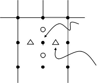
Under normal circumstances, the curvature term, which is a directional diffusion, does not suffer from overshooting; it can be computed directly from firstand second-order derivatives of φ using central difference schemes. However, we have found that central differences do introduce instabilities when computing flows that rely on quantities other than the mean curvature. Therefore, we use the method of differences of normals [101,102] in lieu of central differences. The strategy is to compute normalized gradients at staggered grid points and take the difference of these staggered normals to get centrally located approximations to N (as in Fig. 8.20). The normal projection operator n n is computed with gradient estimates from central differences. The resulting curvatures are
q-1 |
n[p,q |
-1] |
|
|
||
|
N computed as |
|||||
|
|
|
|
|
||
|
|
|
|
|
||
|
|
|
|
|
difference of normals at |
|
n[p-1,q] |
|
|
|
n[p,q] |
original grid location |
|
|
|
|
|
|
||
|
|
|
|
|
|
|
|
|
|
|
|
|
|
|
|
|
|
|
|
|
q
n[p,q]
|
|
|
Staggered normals |
q+1 |
|
|
|
|
|
computed using 6 |
|
|
|
|
|
|
p |
|
neighbors (18 in 3D) |
p-1 |
p+1 |
||
Figure 8.20: The shape matrix B is computed by using the differences of stag-
gered normals.
Level Set Segmentation of Biological Volume Datasets |
461 |
treated as speed terms (motion in the normal direction), and the associated gradient magnitude is computed using the up-wind scheme.
8.6.4.2 Sparse-Field Method
The computational burden associated with solving the 3D, second-order, nonlinear level set PDE is significant. For this reason several papers [34, 35] have proposed narrow-band methods, which compute solutions only for a relatively small set of pixels in the vicinity of k level set. The authors [36] have proposed a sparse-field algorithm, which uses an approximation to the distance transform and makes it feasible to recompute the neighborhood of the level set model at each time step. It computes updates on a band of grid points, called the active set, that is one point wide. Several layers around this active set are updated in such a way as to maintain a neighborhood in order to calculate derivatives. The position of the surface model is determined by the set of active points and their values.
8.6.4.3 Incremental Projection Updates
The tomographic surface reconstruction problem entails an additional computational burden, because the measured data must be compared to the projected model at each iteration. Specifically, computing pij can be a major bottleneck. Computing this term requires recomputing the sinogram of the surface/object model as it moves. In the worst case, we would reproject the entire model every iteration.
To address this computational concern, we have developed the method of incremental projection updates (IPU). Rather than fully recompute p at every iteration, we maintain a current running version of p and update it to reflect the changes in the model as it deforms. Changes in the model are computed only on a small set of grid points in the volume, and therefore the update time is proportional to the area of the surface, rather than the size of the volume it encloses.
The IPU strategy works with the the sparse-field algorithm as follows. At each iteration, the sparse-field algorithm updates only the active layer (one voxel wide) and modifies the set of active grid points as the surface moves. The incremental projection update strategy takes advantage of this to selectively update
462 |
Breen, Whitaker, Museth, and Zhukov |
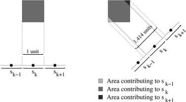
Figure 8.21: A weighting coefficient for each voxel determines the portions of the discrete sinogram influenced by incremental changes to a grid point.
the model projection to reflect those changes. At each iteration, the amount of change in an active point’s value determines the motion of that particular surface point as well as the percentage of the surrounding voxel that is either inside or outside of the surface. By the linearity of projection, we can map these changes in the object shape, computed at grid points along the surface boundary, back into the sinogram space and thereby incrementally update the sinogram. Note that each 3D grid point has a weighting coefficient (these are precomputed and fixed), which is determined by its geometric mapping of the surrounding voxel back into the sinogram, as in Fig. 8.21. In this way the IPU method maintains subvoxel accuracy at a relatively low computational cost.
8.6.4.4 Initialization
The deformable model fitting approach requires an initial model, i.e. φ(x, t = 0). This initial model should be obtained using the “best” information available prior to the surface fitting. In some cases this will mean thresholding a grayscale reconstruction, such as FBP, knowing that it has artifacts. In practice the initial surface estimate is impacted by the reconstruction method and the choice of threshold, and because we perform a local minimization, these choices can affect the final result. Fortunately, the proposed formulation is moderately robust with respect to the initial model, and our results show that the method works well under a range of reasonable initialization strategies.
Level Set Segmentation of Biological Volume Datasets |
463 |
Specimen |
|
|
Contrast |
+90 deg. |
|
Agent |
||
|
||
Detector |
|
|
2D Images |
Data |
|
|
Available |
|
Emitter |
120 –140 |
|
Degrees |
||
|
0 deg. |
|
|
−90 deg. |
|
(a) |
(b) |
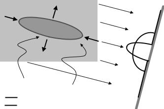
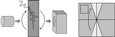
Figure 8.22: (a) Transmission electron microscopy is used to image very small specimens that have been set apart from the substrate by a contrast agent.
(b) TEM imaging technology provides projections over a limited set of angles.
8.6.5 Results
8.6.5.1 Transmission Electron Microscopy
Transmission electron microscopy is the process of using transmission images of electron beams to reveal biological structures on very small dimensions. Typically transmission electron microscopy (TEM) datasets are produced using a dye that highlights regions of interest, e.g. the interior of a microscopic structure, such as a cell (see Fig. 8.22(a)). There are technical limits to the projection angles from which data can be measured. These limits are due to the mechanical apparatus used to tilt the specimens and the trade-off between the destructive effects of electron energy and the effective specimen thickness, which increases with tilt angle. Usually, the maximum tilt angle is restricted to about ±60–70◦. Figure 8.22(b) shows an illustration of the geometry of this limited-angle scenario. The TEM reconstruction problem is further aggravated by the degree of electron scattering, which results in projection images (sinograms) that are noisy relative to many other modalities, e.g. X-ray CT. Finally, due to the flexible nature of biological objects and the imperfections in the tilting mechanism, the objects undergo some movements while being tilted. Manual alignment procedures used to account for this tend to produce small misregistration errors.
We applied the proposed algorithm to 3D TEM data obtained from a 3 MeV electron microscope. This 3D dataset consists of 67 tilt series images, each corresponding to one view of the projection. Each tilt series image is of size 424 × 334. The volume reconstructed by FBP is of size 424 × 424 × 334. Figures 8.23(a)
464 |
Breen, Whitaker, Museth, and Zhukov |
(a) |
(b) |
(c) |
(d) |
(e) |
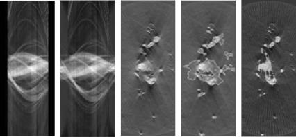
Figure 8.23: 2D slice of dendrite data: (a) sinogram of one slice, (b) sinogram estimated by the proposed method, (c) back projection showing artifacts, (d) initial model obtained by thresholding the back projection (white curve overlaid on the back projection), and (e) final surface estimate.
and (b) show the sinogram corresponding to a single slice of this dataset and the estimate of the same sinogram created by the method. Figure 8.23(e) shows the surface estimate intersecting this slice overlaid on the back projected slice. Some structures not seen in the back projection are introduced in the final estimation, but the orientation of the structures introduced suggests that these are valid features that were lost due to reconstruction artifacts from the FBP. Also, the proposed method captures line-by-line brightness variations in the input sinogram (as explained in Section 8.6.2.1). This suggests that the density estimation procedure is correct.
Figure 8.24 shows the 3D initialization and the final 3D surface estimate. The figure also shows enlarged initial and final versions of a small section of the surface. Computing the surface estimate for the TEM dendrite with 150 iterations took approximately 3 hours on a single 300 MHz processor of a Silicon Graphics Onyx2 workstation. We consider these results positive for several reasons. First, the biology is such that one expects the spines (small protrusions) to be connected to the dendrite body. The proposed method clearly establishes those connections, based solely on consistency of the model with the projected data. The second piece of evidence is the shapes of the spines themselves. The reconstructed model shows the recurrence of a characteristic shape—a long thin spine with a cup-like structure on the end. This characteristic structure, which