Kluwer - Handbook of Biomedical Image Analysis Vol

Whilst geometric or geodesic snakes go a long way in improving on parametric snakes, they still suffer from two significant shortcomings. First, they allow leakage into neighboring image regions when confronted with weak edges; hereafter we refer to this as the weak-edge leakage problem. Second, they may rest at local maxima in noisy image regions. In this chapter, both of these problems are dealt with by introducing diffused region forces into the standard geometric snake formulation. The proposed method is referred to as the region-aided geometric snake or RAGS. It integrates gradient flows with a diffused region vector flow. The gradient flow forces supplant the snake with local object boundary information, while the region vector flow force gives the snake a global view of object boundaries. The diffused region vector flow is derived from the region segmentation map which in turn can be generated from any image segmentation technique. This chapter demonstrates that RAGS can indeed act as a refinement of the results of the initial region segmentation. It also illustrates RAGS’ weak edge leakage improvements and tolerance to noise through various examples. Using color edge gradients, RAGS will be shown to naturally extend to object detection in color images. The partial differential equations (PDEs) resulting from the proposed method will be implemented numerically using level set theory, which enables topological changes to be dealt with automatically.

In Section 10.2 we review the geometric snake model, encompassing its strength and its shortcomings. Section 10.3 provides a brief overview of the geometric GGVF snake, also outlining its shortcomings. The former section is essential as RAGS’ theory is built upon it, and the latter is necessary since we shall make performance comparisons to it. Section 10.4 presents the derivation of the RAGS snake including its level set representation. Then, in Section 10.5, the numerical solutions for obtaining the diffused region force and level set implementation of RAGS are introduced. Section 10.6 describes the extension of RAGS to vector-valued images, again showing the equivalent level set numerical representation. Since RAGS is independent of any particular region segmentation method, its description so far is not affected by the fact that no discussion of region segmentation has yet taken place! This happens next in Section 10.7 where the mean shift algorithm is employed as a typical, suitable method for obtaining a region segmentation map for use with RAGS. Following a brief summary of the RAGS algorithm in Section 10.8, examples and results illustrating the improvements obtained on noisy images and images with weak edges are presented in Section 10.9. This includes an application with

quantitative results comparing the performance of RAGS against the standard geometric snake.

10.2 The Geometric Snake

Geometric active contours were introduced by Caselles et al. [1] and Malladi et al. [2] and are based on the theory of curve evolution. Using a reaction– diffusion model from mathematical physics, a planar contour is evolved with a velocity vector in the direction normal to the curve. The velocity contains two terms: a constant (hyperbolic) motion term that leads to the formation of shocks3 from which more varied and precise representations of shapes can be derived, and a (parabolic) curvature term that smooths the front, showing up significant features and shortening the curve. The geodesic active contour, hereafter also referred to as the standard geometric snake, is now introduced. Let C(x, t) be a 2D active contour. The Euclidean curve shortening flow is given by

where t denotes the time, κ is the Euclidean curvature, and is the unit in-

N

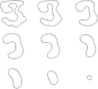
ward normal of the contour. This formulation has many useful properties. For example, it provides the fastest way to reduce the Euclidean curve length in the normal direction of the gradient of the curve. Another property is that it smooths the evolving curve (see Fig. 10.1).

In [3,4], the authors unified curve evolution approaches with classical energy minimization methods. The key insight was to multiply the Euclidean arc length by a function tailored to the feature of interest in the image.

Let I : [0, a] × [0, b] → !+ be an input image in which the task of extracting an object contour is considered. The Euclidean length of a curve C is given by

where ds is the Euclidean arc length. The standard Euclidean metric ds2 = dx2 + dy2 of the underlying space over which the evolution takes place is modified to

3 A discontinuity in orientation of the boundary of a shape; it can also be thought of as a

zero-order continuity.

Figure 10.1: Motion under curvature flow: A simple closed curve will (become smoother and) disappear in a circular shape no matter how twisted it is.

a conformal metric given by

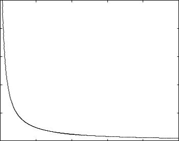
where g(·) represents a monotonically decreasing function such that g(x) → 0 as x → ∞, and g(x) → 1 as x → 0. A typical function for g(x) can be

This is plotted in Fig. 10.2. Using this metric, a new length definition in Riemannian space is given by

1

L! := g(| I(C(q))|)|C (q)|dq. (10.5)

0

Then it is no longer necessary that the minimum path between two points in this metric be a straight line, which is the case in the standard Euclidean metric. The minimum path is now affected by the weighting function g(·). Two distant points in the standard Euclidean metric can be considered to be very close to each other in this metric if there exists a route along which values of g(·) are nearer to zero. The steady state of the active contour is achieved by searching

An example of decreasing function g(x)

for the minimum length curve in the modified Euclidean metric:

1

min g(| I(C(q))|)|C (q)|dq. (10.6)

0

Caselles et al. [4] have shown that this steady state is achieved by determining how each point in the active contour should move along the normal direction in order to decrease the length. The Euler–Lagrange of (10.6) gives the right-hand side of (10.7), i.e., the desired steady state:

Two forces are represented by (10.7). The first is the curvature term multiplied by the weighting function g(·) and moves the curve toward object boundaries constrained by the curvature flow that ensure regularity during propagation. In application to shape modeling, the weighting factor could be an edge indication function that has larger values in homogeneous regions and very small

values on the edges. Since (10.7) is slow, Caselles et al. [4] added a constant in-

flation term to speed up the convergence. The constant flow is given by Ct =

N showing each point on the contour moves in the direction of its normal and on

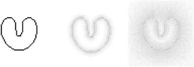
Figure 10.10: Concavity convergence comparison. From left: initial snake, GVF snake result, and GGVF snake result, from [9].

that contours can converge into long, thin boundary indentations. The GGVF preserves clearer boundary information while performing vector diffusion, while the GVF will diffuse everywhere within image. As shown in Fig. 10.10, the GGVF snake shows clear ability to reach concave regions.

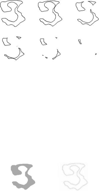
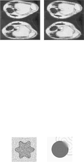
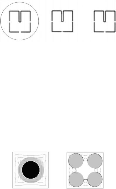
Later in [10], Xu et al. showed the GGVF equivalence in a geometric framework. A simple bimodal region force generated as a two-class fuzzy membership function was added to briefly demonstrate weak-edge leakage handling. The geometric GGVF snake is useful when dealing with boundaries with small gaps. However, it is still not robust to weak edges, especially when a weak boundary is close to a strong edge, the snake readily steps through the weak edge and stops at the strong one. This is illustrated in Fig. 10.11 (left).

A further problem with the GGVF snake is that it does not always allow the detection of multiple objects. These topological problems arise, even though

Figure 10.11: GGVF weaknesses. Left: The GGVF snake steps through a weak edge toward a neighboring strong one (final snake in white). Right: It also can encounter topological problems (final snake in black). The evolving snake is shown in a lighter color in both cases.