556
its squared norm given by
d 2 = 2 2 ∂ ∂ duiduj .
i=1 j=1 ∂ui ∂uj
Using standard Riemannian geometry notation, let sij = ∂
∂ui
|
|
T |
|
|
|
2 |
2 |
|
du1 |
|
s11 |
s12 |
du1 |
d 2 = i 1 j |
|
|
|
= |
1 sij duiduj = du2 |
s21 |
s22 |
du2 |
= |
|
|
|
|
|
|
Xie and Mirmehdi
(10.27)
·∂ , such that
∂uj
.(10.28)
For a unit vector v = (cos θ , sin θ ), then d 2(v) indicates the rate of change of the image in the direction of v. The extrema of the quadratic form are obtained in the directions of the eigenvectors of the metric tensor sij , and the corresponding eigenvalues are
|
|
s11 + s22 ± |
|
|
|
|
λ |
(s11 − s22)2 + 4s122 |
|
(10.29) |
|
2 |
|
± = |
|
|
with eigenvectors (cos θ±, sin θ±) where the angles θ± are given by
θ+ = |
1 |
arctan |
2s12 |
|
2 |
s11 −s22 |
. |
(10.30) |
θ− = θ+ + π2 |
|
The maximal and minimal rates of change are the λ+ and λ− eigenvalues respectively, with corresponding directions of change being θ+ and θ−. The strength of an edge in a vector-valued case is not given simply by the rate of maximal change λ+, but by the difference between the extrema. Hence, a good approximation function for the vector edge magnitude should be based on f = f (λ+, λ−). Now RAGS can be extended to the region-aided geometric color snake by selecting an appropriate edge function fcol. The edge stopping function gcol is defined such that it tends to 0 as fcol → ∞. The following functions can be used (cf. (10.9)):
fcol = λ+ − λ− and gcol = |
1 |
. |
(10.31) |
1 + fcol |
Then replacing gcol(·) for the edge stopping term g(·) in (10.17), we have the color RAGS snake:
Ct |
= |
[gcol( |
| |
| |
)(κ |
+ |
α) |
− |
gcol( |
| |
| |
) |
· N + |
β R˜ |
· N N |
(10.32) |
|
|
I |
|
|
|
I |
|
] . |
A Region-Aided Color Geometric Snake |
557 |
Finally, its level set representation is also given by replacing gcol(·) for g(·) in (10.21):
˜ |
(10.33) |
φt = gcol(| I|)(κ + α)| φ| + gcol(| I|) · φ − β R · φ. |
10.7 The Mean Shift Algorithm
This section can be skipped without loss of continuity. Its topic is the process of generating the image region segmentation map S which is then used as described in Section 10.4.2. The reader can assume it is available and skip to the next section.
An essential requisite for RAGS is a segmentation map of the image. This means that RAGS is independent of any particular segmentation technique as long as a region map is produced; however, it is dependent on its representational quality. In this section, the mean shift algorithm is reviewed as a robust feature space analysis method which is then applied to image segmentation. It provides very reasonable segmentation maps and has extremely few parameters that require tuning.
The concept underlying the nonparametric mean shift technique is to analyze the density of a feature space generated from some input data. It aims to delineate dense regions in the feature space by determining the modes of the unknown density, i.e. first the data is represented by local maxima of an empirical probability density function in the feature space and then its modes are sought. The denser regions are regarded as significant clusters. Comaniciu et al. [13, 20] have recently provided a detailed analysis of the mean shift approach, including the review below, and presented several applications of it in computer vision, e.g. for color image segmentation.
We now briefly present the process of density gradient estimation. Consider a set of n data points {xi}i=1,...,n in the d-dimensional Euclidean space Rd. Also consider the Epanechnikov kernel, an optimum kernel yielding minimum mean integrated square error:
K (x) = |
|
1 |
(d |
+ |
2)(1 |
− |
xT x), if xT x < 1 |
|
|
2Z |
(10.34) |
0, d |
|
otherwise , |
where Zd is the volume of the unit d-dimensional sphere. Using K (x) and window radius h, the multivariate kernel density estimate on the point x is
|
|
|
|
|
|
fˆ(x) |
1 |
n |
|
x − xi |
|
|
= nhd i=1 |
|
h |
|
The estimate of the density gradient can be defined as the gradient of the kernel density estimate since a differentiable kernel is used:
|
|
|
|
≡ |
|
|
= nhd |
i=1 |
|
|
|
h |
|
|
|
|
|
|
|
|
|
|
|
|
|
|
|
|
|
|
|
|
|
|
ˆ f (x) |
|
fˆ(x) |
|
1 |
n |
|
|
x − xi |
|
|
|
|
|
|
|
|
|
|
|
|
K |
|
. |
(10.36) |
Applying (10.34) to (10.36), we obtain |
|
|
|
|
|
|
|
ˆ |
f (x) |
|
nx |
|
d + 2 |
|
1 |
|
[x |
x] , |
|
(10.37) |
|
|
= n(hd Zd) h2 |
|
nx xi Hh(x) |
i − |
|
|
|
where the region Hh(x) is a hypersphere of radius h and volume hd Zd, centered on x, and containing nx data points. The sample mean shift is the last term in (10.37)
|
|
|
|
|
|
|
1 |
|
|
|
|
[xi − x]. |
(10.38) |
|
|
Mh(x) ≡ |
|
|
|
|
|
|
|
nx |
|
|
|
|
|
|
|
|
|
|
|
|
|
|
H (x) |
|
|
|
|
|
|
|
|
|
|
|
|
|
|
xi h |
|
|
|
|
|
|
The quantity |
nx |
is the kernel density estimate fˆ(x) computed with the hy- |
d |
|
n(h Zd ) |
|
|
|
|
|
|
|
|
|
|
|
|
|
|
|
|
|
persphere Hh(x), and thus (10.37) can be rewritten as |
|
|
|
ˆ |
f (x) |
= |
|
fˆ(x) |
d + 2 |
M |
|
(x), |
(10.39) |
|
|
|
|
|
|
|
|
|
|
|
|
|
|
|
|
|
h2 |
h |
|
|
|
which can be rearranged as |
|
|
|
|
|
|
|
|
|
|
|
|
|
|
|
|
|
|
|
|
|
|
|
|
|
|
2 |
|
ˆ |
|
|
|
|
|
|
|
M |
|
(x) |
|
|
|
h |
|
f (x) |
. |
(10.40) |
|
|
|
|
h |
|
|
= d + 2 |
fˆ(x) |
|
|
|
Using (10.40), the mean shift vector provides the direction of the gradient of the density estimate at x which always points toward the direction of the maximum increase (in the density). Hence, it converges along a path leading to a mode of the density.
In [13], Comaniciu et al. performed the mean shift procedure for image segmentation in a joint domain, the image (spatial) domain, and color space (range) domain. The spatial constraints were then inherent in the mode searching procedure. The window radius is the only significant parameter in their segmentation scheme. A small window radius results in oversegmentation (i.e. larger number of clusters), and a large radius produces undersegmentation (yielding a smaller
A Region-Aided Color Geometric Snake |
559 |
number of clusters). In this work, the performance of RAGS will be demonstrated on both the undersegmentation and oversegmentation resolutions of Comaniciu and Meer’s work. In either case, the result of the mean shift procedure is the region segmentation map S which is passed to RAGS for generating
˜
the diffused region boundary map R.
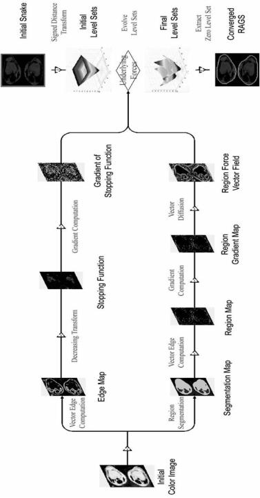
10.8 A Summary of the RAGS Algorithm
The color RAGS algorithm is now reviewed with the aid of Fig. 10.14. Given the input color image, two streams of processing can begin concurrently.
In the first stream, the vector gradient is computed to provide the edge function f , which is then used in (10.9) to yield the decreasing function g, followed by g. Function g will act as spatial weights for the snake curvature force and constant force, and g will contribute to the underlying doublet attraction force.
In the second stream, a region segmentation map S is produced by applying any reasonable segmentation technique, e.g. the mean shift algorithm. From it, region map R can then be generated using vector gradients. Gradient of the region map R provides R, which imposes region forces immediate to region boundaries. These region forces are then diffused by
˜
solving (10.10), resulting in a region force vector field R.
Thus, all the underlying velocity fields and the weighting function g are ready and prepared. Then we can generate initial level sets based on an initial snake using the distance transform and evolve the level sets according to all force fields (rightmost part of Fig. 10.14). The curvature force and constant force adaptively change with the level set snake. Along with the static forces, they are numerically solved using the principles described in Section 10.5.2 with the solutions given in Appendix A. After the level set evolves to a steady state, the final snake is easily obtained by extracting the zero level set.
10.9 Experiments and Results
In this section we present results that show improvements over either the standard geometric snake or the geometric GGVF snake or both, and mainly in
Figure 10.14: RAGS processing schema (color slide).
A Region-Aided Color Geometric Snake |
561 |
images where there are weak edges or noisy regions preventing the aforementioned snakes to perform at their best. Although GGVFs have been reported only using gray level image gradients, we can also apply them to “color” gradients (obtained as described in Section 10.6), which allows direct comparison with the color RAGS. It must also be noted that the GGVF can sometimes perform better than we have shown in some of the following examples as long as it is initialized differently, i.e. much closer to the desired boundary. In all the experiments, we have initiated the geometric, GGVF, and RAGS snakes at the same starting position, unless specifically stated.
10.9.1 Preventing Weak-Edge Leakage
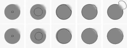
We first illustrate the way weak-edge leakage is handled on a synthetic image. The test object is a circular shape with a small blurred area on the upper right boundary as shown in Fig. 10.15.
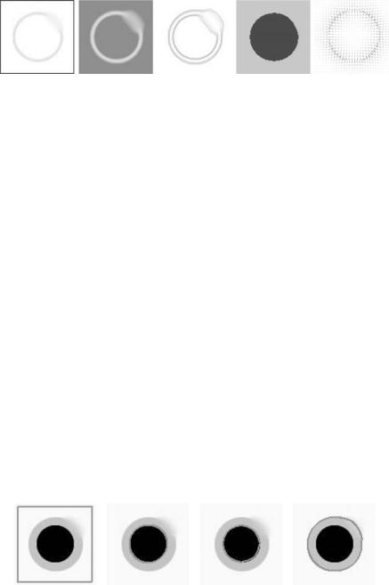
The standard geometric snake steps through the weak edge because the intensity changes so gradually that there is no clear boundary indication in the edge map. The RAGS snake converges to the correct boundary since the extra diffused region force delivers useful global information about the object boundary and helps prevent the snake from stepping through. Figure 10.16 shows, for the test object in Fig. 10.15, the edge map, the stopping function g(·), its gradient magnitude | g(·)|, the region segmentation map S, and the
˜
vector map of the diffused region force R.
Figure 10.15: Weak-edge leakage testing on a synthetic image. Top row: geodesic snake steps through. Bottom row: RAGS snake converges properly using its extra region force.
Figure 10.16: Diffused region force on weak edge. From left: the edge map, the stopping function g(·) of edge map, the magnitude of its gradient g(·), the
˜
region segmentation map, and the vector map of the diffused region force R.
10.9.2 Neighboring Weak/Strong Edges
The next experiment is designed to demonstrate that both the standard geometric snake and the GGVF snake readily step through a weak edge to reach a neighboring strong edge. The test object in Fig. 10.17 contains a prominent circle inside a faint one. The presence of the weaker edge at the outer boundary is detected only by the RAGS snake. The geodesic snake fails because the weaker outer boundary allows the whole snake to leak through (similar to but in the opposite direction of propagation in Fig. 10.15). The GGVF snake fails due to the strong gradient vector force caused by the inner object boundary. Practical examples of this can also be observed in most of the real images shown later, such as Figs 10.20 and 10.26.
10.9.3 Testing on Noisy Images
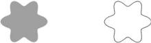
We also performed comparative tests to examine and quantify the tolerance to noise for the standard geometric, the geometric GGVF, and the RAGS snakes. For this a harmonic shape was used as shown in Fig. 10.18. It was generated
Figure 10.17: Strong neighboring edge leakage. From left: initial snake, geodesic snake steps through weak edge in top right of outer boundary, GGVF is attracted by the stronger inner edge, and RAGS snake converges properly using extra region force.
A Region-Aided Color Geometric Snake |
563 |
Figure 10.18: A shape and its boundary (a harmonic curve).
using
r = a + b cos(mθ + c), |
(10.41) |
where r is the length from any edge point to the center of the shape, a, b, and c remain constant, and m can be used to produce different numbers of ‘bumps’; in this case m = 6. We added varying amounts of noise and measured the accuracy of fit (i.e. boundary description) after convergence. The accuracy was computed using maximum radial error (MRE), i.e. the maximum distance in the radial direction between the true boundary and each active contour.
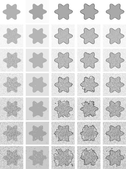
Impulse noise was added to the original image from 10% to 60% as shown in the first column of Fig. 10.19. The region segmentation data used for RAGS is in the second column (without any post-processing to close gaps, etc.). The third, fourth, and fifth columns show the converged snake for the standard geometric, the GGVF, and RAGS snakes respectively. A simple subjective examination clearly demonstrates the superior segmentation quality of the proposed snake. The initial state for the standard geometric and RAGS snakes is a square at the edge of the image, while for the GGVF it is set close to the true boundary to ensure better convergence. At low percentages of noise, all snakes could find the boundary accurately enough. However, at increasing noise levels (>20%), more and more local maxima appear in the gradient flow force field, which prevent the standard geometric and GGVF snakes from converging to the true boundaries. The RAGS snake has a global view of the noisy image and the underlying region force pushes it toward the boundary. The MRE results are shown in Table 10.1. These verify RAGS error values to be consistently and significantly lower than the other two snake types for noise levels >10%.
10.9.4 Results on gray level images
Figures 10.20–10.22 demonstrate RAGS in comparison to the standard geometric and GGVF snakes on various gray level images. Figure (10.20) shows a good example of weak-edge leakage on the lower side of the object of interest. While
Figure 10.19: Shape recovery in noisy images. (Column 1) original image with various levels of added Gaussian noise [0%, 10%, . . . , 60%], (column 2) the region maps later diffused by RAGS, (column 3) standard geometric snake results, (column 4) GGVF snake results, and (column 5) RAGS results.
A Region-Aided Color Geometric Snake |
|
565 |
|
Table 10.1: MRE comparison for the harmonic shapes in |
|
Fig. 10.19 |
|
|
|
|
|
|
|
|
|
|
|
|
Standard geometric |
GGVF |
RAGS |
|
% noise |
snake error |
snake error |
snake error |
|
|
|
|
|
|
0 |
2.00 |
2.00 |
2.00 |
|
10 |
2.23 |
2.24 |
2.00 |
|
20 |
5.00 |
7.07 |
4.03 |
|
30 |
10.00 |
16.03 |
3.41 |
|
40 |
16.16 |
21.31 |
5.22 |
|
50 |
15.81 |
21.00 |
5.38 |
|
60 |
28.17 |
20.10 |
5.83 |
|
|
|
|
|
|
|
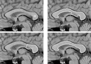
RAGS does extremely well here, the geometric snake leaks through and the GGVF snake leaks and fails to progress at all in the narrow object. In Fig. 10.21, RAGS achieves a much better overall fit than the other snakes, particularly in the lower regions of the right-hand snake and the upper-right regions of the lefthand snake. In Fig. 10.22, again RAGS manages to segment the desired region much better than the standard geometric and the GGVF snakes. Note the stan-
Figure 10.20: Brain MRI (corpus callosum) image. Top row: initial snake, standard geometric snake. Bottom row: GGVF snake and RAGS snake (original image courtesy of GE Medical Systems).