

Intermediate Physics for Medicine and Biology - Russell K. Hobbie & Bradley J. Roth
.pdfAppendix F
Linear Di erential Equations with Constant Coe cients
The equation
dy |
+ by = a |
(F.1) |
|
dt |
|||
|
|
is called a linear di erential equation because each term involves only y or its derivatives [not y(dy/dt) or (dy/dt)2, etc.]. A more general equation of this kind has the form
is called the characteristic equation of this di erential equation. It can be written in a much more compact form using summation notation:
N
bnsn = 0, |
(F.5) |
n=0
dN y |
|
dN −1y |
dy |
+ b0y = f (t). (F.2) |
|
|
+ bN −1 |
|
+ · · · + b1 |
|
|
dtN |
dtN −1 |
dt |
|||
The highest derivative is the N th derivative, so the equation is of order N . It has been written in standard form by dividing through by any bN that was there originally, so that the coe cient of the highest term is one. If all the b’s are constants, this is a linear di erential equation with constant coe cients. The right-hand side may be a function of the independent variable t, but not of y. If f (t) = 0, it is a homogeneous equation; if f (t) is not zero, it is an inhomogeneous equation.
Consider first the homogeneous equation
dN y |
+ bN −1 |
dN −1y |
+ · · · + b1 |
dy |
+ b0y = 0. (F.3) |
dtN |
dtN −1 |
dt |
The exponential est (where s is a constant) has the property that d(est)/dt = sest, d2(est)/dt2 = s2est, dn(est)/dtn = snest. The function y = Aest satisfies Eq. F.3 for any value of A and certain values of s. The equation becomes
A sN est + bN −1sN −1est + · · · + b1sest + b0est = 0, A sN + bN −1sN −1 + · · · + b1s + b0 est = 0.
This equation is satisfied if the polynomial in parentheses is equal to zero. The equation
sN + bN −1sN −1 + · · · + b1s + b0 = 0 (F.4)
with bN = 1.
For Eq. F.1, the characteristic equation is s + b = 0 or
s = −b, and a solution to the homogeneous equation is y = Ae−bt.
If the characteristic equation is a polynomial, it can have up to N roots. For each distinct root sn, y = Anesn t is a solution to the di erential equation. (The question of solutions when there are not N distinct roots will be taken up below.) This is still not the solution to the equation we need to solve. However, one can prove1 that the most general solution to the inhomogeneous equation consists of the homogeneous solution,
N
y = Anesn t,
n=1
plus any solution to the inhomogeneous equation. The values of the arbitrary constants An are picked to satisfy some other conditions that are imposed on the problem. If we can guess the solution to the inhomogeneous equation, that is fine. However we get it, we need only one such solution to the inhomogeneous equation. We will not prove this assertion, but we will apply it to the firstand second-order equations and see how it works.
1See, for example, G. B. Thomas. Calculus and Analytic Geometry, Reading, MA, Addison-Wesley (any edition).

558 Appendix F. Linear Di erential Equations with Constant Coe cients
F.1 First-order Equation
The homogeneous equation corresponding to Eq. F.1 has solution y = Ae−bt. There is one solution to the inhomogeneous equation that is particularly easy to write down: when y is constant, with the value y = a/b, the time derivative vanishes and the inhomogeneous equation is satisfied. The most general solution is therefore of the
form
y = Ae−bt + ab .
If the initial condition is y(0) = 0, then A can be deter-
mined from 0 = Ae−b0 + a/b. Since e0 |
= 1, this gives |
||
A = −a/b. Therefore |
|
||
y = |
a |
1 − e−bt . |
(F.6) |
b |
|||
A physical example of this is given in Sec. 2.7.
F.2 Second-order Equation
The second-order equation
d2y |
|
dy |
|
|
|
+ b1 |
|
+ b0y = 0 |
(F.7) |
dt2 |
|
|||
|
dt |
|
||
has a characteristic equation s2 + b1s + b0 = 0 with roots
s = |
−b1 ± # |
b12 − 4b0 |
. |
(F.8) |
|
2 |
|||||
|
|
|
|||
This equation may have no, one, or two solutions.
If it has two solutions s1 and s2, then the general solution of the homogeneous equation is y = A1es1t + A2es2t.
If b21 − 4b0 is negative, there is no solution to the equation for a real value of s. However, a solution of the form y = Ae−αt sin(ωt + φ) will satisfy the equation. This can be seen by direct substitution. Di erentiating this twice shows that
|
dy |
= |
− |
αAe−αt sin(ωt + φ) + ωAe−αt cos(ωt + φ), |
|||
|
dt |
||||||
|
|
|
|
|
|
||
d2y |
|
= |
α2Ae−αtsin(ωt + φ) |
− |
2αωAe−αt cos(ωt + φ) |
||
dt2 |
|
||||||
|
|
|
|
|
|||
− ω2Ae−αt sin(ωt + φ).
If these derivatives are substituted in Eq. F.7, one gets the following results. The terms are written in two columns. One column contains the coe cients of terms with sin(ωt + φ), and the other column contains the co- e cients of terms with cos(ωt + φ). The rows are labeled on the left by which term of the di erential equation they came from.
Term |
Coe cients |
|
|
sin(ωt + φ) |
cos(ωt + φ) |
d2y/dt2 |
α2 − ω2 |
−2αω |
b1(dy/dt) |
−b1α |
b1ω |
b0y |
b0 |
0 |
The only way that the equation can be satisfied for all times is if the coe cient of the sin(ωt + φ) term and the coe cient of the cos(ωt + φ) term separately are equal to zero. This means that we have two equations that must be satisfied (call b0 = ω02):
2αω = b1ω,
α2 − ω2 − b1α + ω02 = 0.
From the first equation 2α = b1, while from this and the second, α2 − ω2 − 2α2 + ω02 = 0, or ω2 = ω02 − α2. Thus, the solution to the equation
|
d2y |
+ 2α |
dy |
+ ω2y = 0 |
(F.9) |
|
|
|
|||
|
dt2 |
|
dt |
0 |
|
|
|
|
|
||
is |
|
|
|
|
|
|
y = Ae−αt sin(ωt + φ) |
(F.10a) |
|||
where |
|
|
|
|
|
ω2 = ω02 − α2, α < ω0. |
(F.10b) |
||||
Solution F.10 is a decaying exponential multiplied by a sinusoidally varying term. The initial amplitude A and the phase angle φ are arbitrary and are determined by other conditions in the problem. The constant α is called the damping. Parameter ω0 is the undamped frequency, the frequency of oscillation when α = 0. ω is the damped frequency.
When the damping becomes so large that α = ω0, then the solution given above does not work. In that case, the solution is given by
y = (A + Bt)e−αt, α = ω0. |
(F.11) |
This case is called critical damping and represents the case in which y returns to zero most rapidly and without multiple oscillations. The solution can be verified by substitution.
If α > ω0, then the solution is the sum of the two exponentials that satisfy Eq. F.8:
y = Ae−at + Be−bt, |
(F.12a) |
||||||
where |
|
|
|
|
|
|
|
a = α + , |
α2 − ω02 |
, |
(F.12b) |
||||
|
|
|
|||||
b = α − , |
α2 − ω02 |
. |
(F.12c) |
||||
When α = 0, the equation is |
|
||||||
|
d2y |
+ ω2y = 0. |
(F.13) |
||||
|
|
||||||
|
dt2 |
0 |
|
|
|
||
|
|
|
|
|
|
|
|
The solution may be written either as |
|
||||||
y = C sin(ω0t + φ) |
(F.14a) |
||||||
or as |
|
|
|
|
|
|
|
y = A cos(ω0t) + B sin(ω0t). |
(F.14b) |
||||||
Problems 559
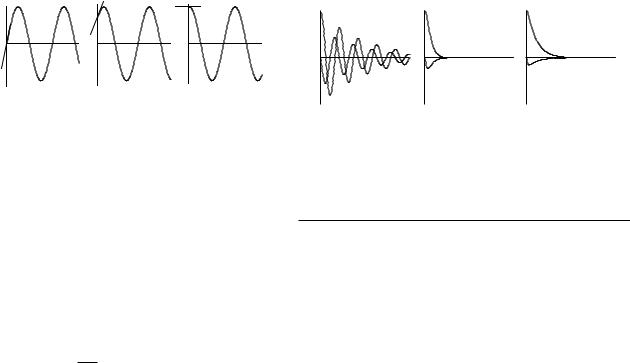
Underdamped |
t |
Critically damped |
t |
Overdamped |
t |
FIGURE F.1. Di erent starting points on the sine wave give di erent combinations of the initial position and the initial velocity.
The simplest physical example of this equation is a mass on a spring. There will be an equilibrium position of the mass (y = 0) at which there is no net force on the mass. If the mass is displaced toward either positive or negative y, a force back toward the origin results. The force is proportional to the displacement and is given by F = −ky. The proportionality constant k is called the spring constant. Newton’s second law, F = ma, is m(d2y/dt2) = −ky or, defining ω02 = k/m,
d2y + ω2y = 0. dt2 0
This (as well as the equation with α = 0) is a second-order di erential equation. Integrating it twice introduces two constants of integration: C and φ, or A and B. They are usually found from two initial conditions. For the mass on the spring, they are often the initial velocity and initial position of the mass.
The equivalence of the two solutions can be demonstrated by using Eqs. F.14a and a trigonometric identity to write C sin(ω0t + φ) = C[sin ω0t cos φ + cos ω0t sin φ]. Comparison with Eq. F.14b shows that B = C cos φ, A = C sin φ. Squaring and adding these gives C2 = A2 + B2, while dividing one by the other shows that tan φ = A/B.
Changing the initial phase angle changes the relative values of the initial position and velocity. This can be seen from the three plots of Fig. F.1, which show phase angles 0, π/4, and π/2. When φ = 0, the initial position is zero, while the initial velocity has its maximum value. When φ = π/4, the initial position has a positive value, and so does the initial velocity. When φ = π/2 the initial position has its maximum value and the initial velocity is zero. The values of A and B are determined from the initial position and velocity. At t = 0, Eq. F.14b and its derivative give y(0) = A, dy/dt(0) = ω0B.
The term in the di erential equation equal to 2α(dy/dt) corresponds to a drag force acting on the mass and damping the motion. Increasing the damping coefficient α increases the rate at which the oscillatory behavior decays. Figure F.2 shows plots of y and dy/dt for di erent values of α.
FIGURE F.2. Plot of y(t) (solid line) and dy/dt (dashed line) for di erent values of α.
TABLE F.1. Solutions of the harmonic oscillator equation.
d2y |
dy |
+ ω2y = 0 |
|||
|
|
+ 2α |
|
||
|
|
|
|||
|
dt2 |
|
dt |
|
0 |
|
|
|
|
||
Case |
Criterion |
Solution |
|||
|
|
|
|
||
Underdamped |
α < ω0 |
|
y = Ae−αt sin(ωt + φ) |
||
|
|
|
|
|
ω2 = ω02 − α2 |
Critically damped |
α = ω0 |
|
y = (A + Bt)e−αt |
||
Overdamped |
α > ω0 |
|
y = Ae−at + Be−bt |
||
|
|
|
|
|
a = α + (α2 − ω02)1/2 |
|
|
|
|
|
b = α − (α2 − ω02)1/2 |
The second-order equation we have just studied is called the harmonic oscillator equation. Its solution is needed in Chap. 8 and is summarized in Table F.1.
Problems
Problem 1 From Eq. F.14 with ω0 = 10, find A, B, C, and φ for the following cases:
(a)y(0) = 5, (dy/dt)(0) = 0.
(b)y(0) = 5, (dy/dt)(0) = 5.
(c)y(0) = 0, (dy/dt)(0) = 50.
(d)What values of A, B, and C would be needed to have the same φ as in case (b) and the same amplitude as in case (a)?
Problem 2 |
Verify Eq. |
F.11 |
in |
the |
critically damped |
|||||
case. |
|
|
|
|
|
|
|
|
|
|
Problem 3 |
Find the general solution of the equation |
|||||||||
d2y |
dy |
2 |
$ |
0, |
t |
≤ |
0 |
|||
|
|
+ 2α |
|
+ ω0 y = |
|
2 |
, t |
|
||
|
dt2 |
|
|
|
||||||
|
|
dt |
|
|
ω0 y0 |
≥ 0 |
||||
subject to the initial conditions y(0) = 0, |
(dy/dt)(0) = 0 |
|||||||||
(a)for critical damping, α = ω0,
(b)for no damping, and
(c)for overdamping, α = 2ω0.

Appendix G
The Mean and Standard Deviation
TABLE G.1. Quiz scores.
Student No. |
Score |
Student No. |
Score |
1 |
80 |
16 |
71 |
2 |
68 |
17 |
83 |
3 |
90 |
18 |
88 |
4 |
72 |
19 |
75 |
5 |
65 |
20 |
69 |
6 |
81 |
21 |
50 |
7 |
85 |
22 |
81 |
8 |
93 |
23 |
94 |
9 |
76 |
24 |
73 |
10 |
86 |
25 |
79 |
11 |
80 |
26 |
82 |
12 |
88 |
27 |
78 |
13 |
81 |
28 |
84 |
14 |
72 |
29 |
74 |
15 |
67 |
30 |
70 |
|
|
|
|
In many measurements in physics or biology there may be several possible outcomes to the measurement. Different values are obtained when the measurement is repeated. For example, the measurement might be the number of red cells in a certain small volume of blood, whether a person is right-handed or left-handed, the number of radioactive disintegrations of a certain sample during a 5-min interval, or the scores on a test.
Table G.1 gives the scores on an examination administered to 30 people. These results are also plotted as a histogram in Fig. G.1.
The table and the histogram give all the information that there is to know about the experiment unless the result depends on some variable that was not recorded, such as the age of the student or where the student was sitting during the test.
In many cases the frequency distribution gives more information than we need. It is convenient to invent some quantities that will answer the questions: Around what values do the results cluster? How wide is the distribution of results? Many di erent quantities have been invented for answering these questions. Some are easier to calculate or have more useful properties than others.
The mean or average shows where the distribution is centered. It is familiar to everyone: add up all the scores and divide by the number of students. For the data given above the mean is x = 77.8.
It is often convenient to group the data by the value obtained, along with the frequency of that value. The data of Table G.1, are grouped this way in Table G.2. The mean is calculated as
|
|
1 |
i fixi |
|
||
|
|
|
||||
x = |
|
|
fixi = |
|
, |
|
N |
i fi |
|||||
|
|
|
i |
|
|
|
where the sum is over the di erent values of the test scores that occur. For the example in Table G.2, the sums are
i fi = 30, i fixi = 2335, so x = 2335/30 = 77.8. If a large number of trials are made, fi/N can be called the
f |
6 |
|
|
|
|
|
|
|
|
|
|
|
|
|
|
|
|
|
|
|
|
|
|
|
|
|
|
|
score, |
4 |
|
|
|
|
|
|
|
|
|
|
|
|
|
|
|
_ |
σ |
|
|||||||||
|
|
|
|
|
|
|
|
|
|
|
|
|
|
|
|
|
σ x |
|
||||||||||
of |
5 |
|
|
|
|
|
|
|
|
|
|
|
|
|
|
|
|
|
|
|
|
|
|
|
|
|
|
|
3 |
|
|
|
|
|
|
|
|
|
|
|
|
|
|
|
|
|
|
|
|
|
|
|
|
|
|
|
|
|
|
|
|
|
|
|
|
|
|
|
|
|
|
|
|
|
|
|
|
|
|
|
|
|
|
|
||
|
|
|
|
|
|
|
|
|
|
|
|
|
|
|
|
|
|
|
|
|
|
|
|
|
|
|
||
|
|
|
|
|
|
|
|
|
|
|
|
|
|
|
|
|
|
|
|
|
|
|
|
|
|
|
||
Frequency |
|
|
|
|
|
|
|
|
|
|
|
|
|
|
|
|
|
|
|
|
|
|
|
|
|
|
|
|
|
|
|
|
|
|
|
|
|
|
|
|
|
|
|
|
|
|
|
|
|
|
|
|
|
|
|
||
2 |
|
|
|
|
|
|
|
|
|
|
|
|
|
|
|
|
|
|
|
|
|
|
|
|
|
|
|
|
|
|
|
|
|
|
|
|
|
|
|
|
|
|
|
|
|
|
|
|
|
|
|
|
|
|
|
|
|
|
1 |
|
|
|
|
|
|
|
|
|
|
|
|
|
|
|
|
|
|
|
|
|
|
|
|
|
|
|
|
|
|
|
|
|
|
|
|
|
|
|
|
|
|
|
|
|
|
|
|
|
|
|
|
|
|
|
|
|
0 |
|
|
|
|
|
|
|
|
|
|
|
|
|
|
|
|
|
|
|
|
|
|
|
|
|
|
|
|
|
20 |
40 |
60 |
|
|
80 |
100 |
||||||||||||||||||||
|
0 |
|
|
|||||||||||||||||||||||||
Score, x
FIGURE G.1. Histogram of the quiz scores in Table G.1

562 Appendix G. The Mean and Standard Deviation
TABLE G.2. Quiz scores grouped by score
Score |
Score xi |
Frequency of |
fixi |
number i |
|
score, fi |
|
1 |
50 |
1 |
50 |
2 |
65 |
1 |
65 |
3 |
67 |
1 |
67 |
4 |
68 |
1 |
68 |
5 |
69 |
1 |
69 |
6 |
70 |
1 |
70 |
7 |
71 |
1 |
71 |
8 |
72 |
2 |
144 |
9 |
73 |
1 |
73 |
10 |
74 |
1 |
74 |
11 |
75 |
1 |
75 |
12 |
76 |
1 |
76 |
13 |
78 |
1 |
78 |
14 |
79 |
1 |
79 |
15 |
80 |
2 |
160 |
16 |
81 |
3 |
243 |
17 |
82 |
1 |
82 |
18 |
83 |
1 |
83 |
19 |
84 |
1 |
84 |
20 |
85 |
1 |
85 |
21 |
86 |
1 |
86 |
22 |
88 |
2 |
176 |
23 |
90 |
1 |
90 |
24 |
93 |
1 |
93 |
25 |
94 |
1 |
94 |
|
|
|
|
probability pi of getting result xi. Then |
|
||||
|
|
|
|
= xipi. |
(G.1) |
|
|
x |
|||
|
|
|
|
i |
|
Note that pi = 1. |
|
||||
The average of some function of x is |
|
||||
|
|
= g(xi)pi. |
(G.2) |
||
|
g(x) |
||||
|
|
|
|
i |
|
For example,
x2 = (xi)2pi.
i
The width of the distribution is often characterized by the dispersion or variance:
(∆x)2 |
= |
(x − |
|
)2 |
= pi(xi − |
|
)2. |
(G.3) |
x |
x |
|||||||
|
|
|
|
|
i |
|
||
This is also sometimes called the mean square variation: the mean of the square of the variation of x from the mean. A measure of the width is the square root of this, which is called the standard deviation σ. The need for taking the square root is easy to see since x may have units associated with it. If x is in meters, then the variance has the units of square meters. The width of the distribution in x must be in meters.
A very useful result is
(x − x)2 = x2 − x2.
To prove this, note that (xi − x)2 = x2i − 2xix + x2. The variance is then
(∆x)2 = pix2i − 2 xi x pi + pix2.
i i i
The first sum is the definition of x2. The second sum has a number x in every term. It can be factored in front of the
sum, to make the second term −2x xipi, which is just −2(x)2. The last term is (x)2 pi = (x)2. Combining all three sums gives Eq. G.4. In summary,
σ = |
, |
|
|
|
|
(∆x)2 |
, |
(G.4) |
|||
σ2 = (∆x)2 = (x − x)2 = x2 − x2.
This equation is true as long as the pi’s are accurately known. If the pi’s have only been estimated from N experimental observations, the best estimate of σ2 is N/(N −1) times the value calculated from Eq. G.4.
For the data of Fig. G.1, σ = 9.4. This width is shown along with the mean at the top of the figure.
Problems
Problem 1 Calculate the variance and standard deviation for the data in Table G.2.

Appendix H
The Binomial Probability Distribution
Consider an experiment with two mutually exclusive outcomes that is repeated N times, with each repetition being independent of every other. One of the outcomes is labeled “success”; the other is called “failure.” The experiment could be throwing a die with success being a three, flipping a coin with success being a head, or placing a particle in a box with success being that the particle is located in a subvolume v.
In a single try, call the probability of success p and the probability of failure q. Since one outcome must occur and both cannot occur at the same time,
p + q = 1. |
(H.1) |
Suppose that the experiment is repeated N times. The probability of n successes out of N tries is given by the binomial probability distribution, which is stated here without proof.1 We can call the probability P (n; N ), since it is a function of n and depends on the parameter N . Strictly speaking, it depends on two parameters, N and p: P (n; N, p). It is2
P (n; N ) = P (n; N, p) = |
N ! |
|
pn(1 − p)N −n. |
|
n!(N |
− |
n)! |
||
|
|
|
|
|
(H.2) The factor N !/[n!(N − n)!] counts the number of different ways that one can get n successful outcomes; the probability of each of these ways is pn(1 − p)N −n. In the example of three particles in Sec. 3.1, there are three ways to have one particle in the left-hand side. The particle can be either particle a or particle b or particle c. The factor
1A detailed proof can be found in many places. See, for example, F. Reif (1964). Statistical Physics. Berkeley Physics Course, Vol. 5, New York, McGraw-Hill, p. 67.
2N ! is N factorial and is N (N − 1)(N − 2) · · · 1. By definition, 0! = 1.
gives directly
N ! |
= |
|
3! |
= |
3 × 2 × 1 |
= |
6 |
= 3. |
||
|
|
|
|
|
||||||
n!(N − n)! |
1!2! |
(1)(2 × 1) |
2 |
|||||||
|
|
|
|
|||||||
The remaining factor, pn(1 − p)N −n, is the probability of taking n tries in a row and having success and taking N − n tries in a row and having failure.
The binomial distribution applies if each “try” is independent of every other try. Such processes are called Bernoulli processes (and the binomial distribution is often called the Bernoulli distribution). In contrast, if the probability of an outcome depends on the results of the previous try, the random process is called a Markov process. Although such processes are important, they are more di cult to deal with and are not discussed here.
Some examples of the use of the binomial distribution are given in Chap. 3. As another example, consider the problem of performing several laboratory tests on a patient. In the 1970s it became common to use automated machines for blood-chemistry evaluations of patients; such machines automatically performed (and reported) 6, 12, 20, or more tests on one small sample of a patient’s blood serum, for less cost than doing just one or two of the tests. But this meant that the physician got a large number of results—many more than would have been asked for if the tests were done one at a time. When such test batteries were first done, physicians were surprised to find that patients had many more abnormal tests than they expected. This was in part because some tests were not known to be abnormal in certain diseases, because no one had ever looked at them in that disease. But there still was a problem that some tests were abnormal in patients who appeared to be perfectly healthy.
We can understand why by considering the following idealized situation. Suppose that we do N independent tests, and suppose that in healthy people, the probability that each test is abnormal is p. (In our vocabulary,
564 |
|
Appendix H. The Binomial Probability Distribution |
||||||||||||
|
|
1.0 |
|
|
|
|
|
|
|
|
|
|
|
|
|
|
|
|
|
|
|
|
|
|
|
|
|
|
|
|
|
|
|
|
|
|
|
|
|
|
|
|||
|
|
0.8 |
|
|
|
|
|
34 Clinically normal patients |
|
|||||
|
|
|
|
|
|
|
||||||||
|
|
|
|
|
|
|
|
|
|
|
||||
|
|
|
|
|
|
|
Binomial distribution |
|
|
|||||
|
|
|
|
|
||||||||||
|
|
|
|
|
|
|
|
P(n,12) if p = 0.05 |
|
|
||||
|
patientsof |
0.6 |
|
|
|
|
|
|
|
|
|
|
|
|
|
|
|
|
|
|
|
|
|
|
|
|
|
||
|
Fraction |
|
|
|
|
|
|
|
|
|
|
|
|
|
|
0.4 |
|
|
|
|
|
|
|
|
|
|
|
|
|
|
|
|
|
|
|
|
|
|
|
|
|
|
|
|
|
|
0.2 |
|
|
|
|
|
|
|
|
|
|
|
|
|
|
|
|
|
|
|
|
|
|
|
|
|
|
|
|
|
0.0 |
|
|
|
|
|
|
|
|
|
|
|
|
|
|
|
|
|
|
|
|
|
|
|
|
|
|
|
|
|
|
|
|
|
|
|
|
|
|
|
|
|
|
|
|
|
|
|
|
|
|
|
|
|
|
|
|
|
0 |
1 |
2 |
3 |
Number of abnormal tests
tests. The data have the general features predicted by this simple model.
We can derive simple expressions to give the mean and standard deviation if the probability distribution is binomial. The mean value of n is defined to be
|
|
N |
N |
N !n |
|
|
|
|
|
|
= nP (n; N ) = |
pn(1 |
− |
p)N −n. |
|||
n |
||||||||
|
|
|||||||
|
|
n=0 |
n=0 n!(N − n)! |
|
|
|||
The first term of each sum is for n = 0. Since each term is multiplied by n, the first term vanishes, and the limits of the sum can be rewritten as
N |
N !n |
|
|
|
|
|
pn(1 |
− |
p)N −n. |
||
|
|||||
n=1 n!(N − n)! |
|
|
|||
To evaluate this sum, we use a trick. Let m = n − 1 and M = N − 1. Then we can rewrite various parts of this expression as follows:
FIGURE H.1. Measurement of the probablity that a clinically normal patient having a battery of 12 tests done has n abnormal tests (solid line) and a calculation based on the binomial distribution (dashed line). The calculation assumes that p = 0.05 and that all 12 tests are independent. Several of the tests in this battery are not independent, but the general features are reproduced.
n |
= |
1 |
= |
1 |
, |
|
n! |
(n − 1)! |
m! |
||||
|
|
|
pn = ppm,
N ! = (N )(N − 1)!,
(N − n)! = [N − 1 − (n − 1)]! = (M − m)!.
The limits of summation are n = 1 or m = 0, and n = N or m = M . With these substitutions
having an abnormal test is “success”!). The probability |
|
|
|
|
|
|
|
M |
|
|
|
|
|
|
M ! |
|
|
|
|
|
|
|
|
|
||||||||
|
|
|
|
|
= N p |
|
|
|
|
|
|
pm(1 |
− |
p)M −m. |
||||||||||||||||||
|
|
|
n |
|
|
|
|
|
||||||||||||||||||||||||
of not having the test abnormal is q = 1 − p. In a per- |
|
|
|
|
|
|
|
m=0 |
m!(M − m)! |
|
|
|
|
|
|
|
||||||||||||||||
fect test, p would be 0 for healthy people and would be 1 |
This sum is exactly the sum of a binomial distribution |
|||||||||||||||||||||||||||||||
in sick people; however, very few tests are that discrim- |
||||||||||||||||||||||||||||||||
over all possible values of m and is equal to one. We have |
||||||||||||||||||||||||||||||||
inating. The definition of normal vs abnormal involves |
||||||||||||||||||||||||||||||||
the result that, for a binomial distribution, |
|
|
||||||||||||||||||||||||||||||
a compromise between false positives (abnormal test re- |
|
|
||||||||||||||||||||||||||||||
|
|
|
|
|
|
|
|
|
|
|
|
|
|
|
= N p. |
|
|
|
|
|
|
|
(H.3) |
|||||||||
sults in healthy people) and false negatives (normal test |
|
|
|
|
|
|
|
|
|
|
|
|
|
|
|
|
|
|
|
|
|
|
||||||||||
|
|
|
|
|
|
|
|
|
|
|
|
|
|
n |
|
|
|
|
|
|
|
|||||||||||
results in sick people). Good reviews of this problem have |
This says that the average number of successes is the total |
|||||||||||||||||||||||||||||||
been written by Murphy and Abbey3 and by Feinstein.4 |
||||||||||||||||||||||||||||||||
number of tries times the probability of a success on each |
||||||||||||||||||||||||||||||||
In many cases, p is about 0.05. Now suppose that p is the |
||||||||||||||||||||||||||||||||
try. If 100 particles are placed in a box and we look at half |
||||||||||||||||||||||||||||||||
same for all the tests and that the tests are independent. |
||||||||||||||||||||||||||||||||
the box so that p = |
|
1 , the average number of particles |
||||||||||||||||||||||||||||||
Neither of these assumptions is very good, but they will |
in that half is 100 |
|
|
|
2 |
= 50. If we put 500 particles in |
||||||||||||||||||||||||||
× |
1 |
|||||||||||||||||||||||||||||||
show what the basic problem is. Then, the probability |
|
|
|
|
|
|
|
|
2 |
|
of the box, the average number |
|||||||||||||||||||||
|
|
|
|
|
|
|
|
1 |
|
|||||||||||||||||||||||
|
|
|
|
|
|
the box and look at |
|
|
|
|||||||||||||||||||||||
for all of the N tests to be normal in a healthy patient is |
10 |
|
||||||||||||||||||||||||||||||
of particles in the volume is also 50. If we have 100 000 |
||||||||||||||||||||||||||||||||
given by the binomial probability distribution: |
|
|
||||||||||||||||||||||||||||||
|
|
particles and v/V = p = 1/2000, the average number is |
||||||||||||||||||||||||||||||
|
|
|
|
|
|
|||||||||||||||||||||||||||
P (0; N, p) = |
N ! |
p0qN = qN . |
|
|
still 50. |
|
|
|
|
|
|
|
|
|
|
|
|
|
|
|
|
|
|
|
||||||||
|
|
|
For the binomial distribution, the variance σ2 can be |
|||||||||||||||||||||||||||||
|
|
|
||||||||||||||||||||||||||||||
|
0!N ! |
|
|
expressed in terms of N and p using Eq. G.4. The average |
||||||||||||||||||||||||||||
|
|
|
|
|
|
|||||||||||||||||||||||||||
If p = 0.05, then q = 0.95, and P (0; N, p) = 0.95 |
N |
. Typi- |
of n2 is |
|
|
|
|
|
|
|
|
|
|
|
|
|
|
|
|
|
|
|
||||||||||
|
|
|
|
|
|
|
|
|
|
|
|
|
|
|
|
|
|
|
|
|
|
|
|
|
|
|
||||||
cal values are P (0; 12) = 0.54, and P (0; 20) = 0.36. If the |
|
|
|
|
|
|
|
|
|
|
|
|
|
|
N |
N ! |
|
|
|
|
|
|
||||||||||
|
|
= P (n; N )n2 = |
|
|
|
|
n2pn(1 |
|
p)N −n. |
|||||||||||||||||||||||
|
n2 |
|
|
− |
||||||||||||||||||||||||||||
assumptions about p and independence are right, then |
|
|
|
|
|
|
|
|||||||||||||||||||||||||
|
|
|
|
|
|
|
|
|
|
|
|
|
|
|
n!(N |
− |
n)! |
|
|
|||||||||||||
only 36% of healthy patients will have all their tests nor- |
|
|
n |
|
|
|
|
|
|
n=0 |
|
|
|
|
|
|
|
|||||||||||||||
mal if 20 tests are done. |
|
|
The trick to evaluate this is to write n2 = n(n − 1) + n. |
|||||||||||||||||||||||||||||
Figure H.1 shows a plot of the number of patients in a |
With this substitution we get two sums: |
|
|
|
||||||||||||||||||||||||||||
series who were clinically normal but who had abnormal |
|
|
|
|
|
|
|
N |
|
|
|
|
|
N ! |
|
|
|
|
|
|
|
|
|
|||||||||
|
|
|
|
|
|
|
|
|
|
|
= |
|
|
|
|
|
n(n |
|
1)pnqN −n |
|
||||||||||||
|
|
|
|
|
|
|
|
|
|
n2 |
|
|
|
|
− |
|
||||||||||||||||
|
|
|
|
|
|
|
|
|
|
|
|
|
|
|
|
|
|
|||||||||||||||
3E. A. Murphy and H. Abbey (1967). The normal range—a com- |
|
|
|
|
|
|
|
n=0 n!(N − n)! |
|
|
|
|
|
|
|
|
||||||||||||||||
mon misuse. J. Chronic Dis. 20: 79. |
|
|
|
|
|
|
|
|
|
|
|
|
N |
|
|
N !n |
|
|
|
|
|
|
|
|
|
|||||||
4A. R. Feinstein (1975). Clinical biostatistics XXVII. The de- |
|
|
|
|
|
|
|
+ |
|
|
|
|
|
|
pnqN −n. |
|
|
|||||||||||||||
|
|
|
|
|
|
|
|
|
|
|
|
|
|
|
|
|||||||||||||||||
rangements of the normal range. Clin. Pharmacol. Therap. 15: 528. |
|
|
|
|
|
|
|
|
|
n=0 n!(N − n)! |
|
|
|
|
|
|
||||||||||||||||

|
0.6 |
|
|
|
|
|
1/2 |
0.4 |
|
|
|
|
|
|
|
|
|
|
|
|
[p(1-p)] |
0.2 |
|
|
|
|
|
|
0.0 |
|
|
|
|
|
|
0.0 |
0.2 |
0.4 |
0.6 |
0.8 |
1.0 |
|
|
|
|
p |
|
|
|
FIGURE H.2. Plot of [p(1 − p)]1/2. |
|
||||
The second sum is n = N p. The first sum is rewritten by noticing that the terms for n = 0 and n = 1 both vanish. Let m = n − 2 and M = N − 2:
|
|
|
M |
M ! |
|
|
|
= N p + N (N |
|
1) |
p2pmqM −m |
||
n2 |
− |
|||||
|
||||||
|
|
m=0 m!(M − m)! |
|
|||
= N p + N (N − 1)p2 = N p + N 2p2 − N p2.
Therefore,
(∆n)2 = n2 − n2 = N p − N p2 = N p(1 − p) = N pq.
For the binomial distribution, then,
##
σ = N pq = nq.
The standard deviation for the binomial distribution for fixed p goes as N 1/2. For fixed N , it is proportional
#
to p(1 − p), which is plotted in Fig. H.2. The maximum value of σ occurs when p = q = 12 . If p is very small, the event happens rarely; if p is close to 1, the event nearly always happens. In either case, the variation is reduced. On the other hand, if N becomes large while p becomes
small in such a way as to keep n fixed, then σ increases
√
to a maximum value of n. This variation of σ with N and p is demonstrated in Fig. H.3. Figures H.3(a)–H.3(c) show how σ changes as N is held fixed and p is varied. For N = 100, p is 0.05, 0.5, and 0.95. Both the mean and σ change. Comparing Fig. H.3(b) with H.3(d) shows two di erent cases where n = 50. When p is very small because N is very large in Fig. H.3(d), σ is larger than in Fig. H.3(b).
Problems
Problem 1 Calculate the probability of throwing 0, 1, . . . , 9 heads out of a total of nine throws of a coin.
Problem 2 Assume that males and females are born with equal probability. What is the probability that a couple will have four children, all of whom are girls? The couple has had three girls. What is the probability that they will have a fourth girl? Why are these probabilities so di erent?
|
|
|
|
|
|
|
|
|
|
|
|
|
|
|
|
|
|
|
|
|
|
|
|
|
|
|
Problems |
565 |
||||||||||
0.20 |
|
|
|
|
|
|
|
|
|
|
|
|
|
|
|
|
|
|
|
|
|
|
|
|
|
|
|
|
|
|
|
|
|
|
|
|
|
|
|
|
|
|
|
|
|
|
|
|
(a) |
|
|
|
N = 100 |
|
|
|
|
|
|
|
(c) |
|
|
|
|
||||||||||||
0.15 |
|
|
|
|
|
|
|
|
|
p = 0.05 |
|
|
|
|
|
|
|
|
|
|
|
|
|
p = 0.95 |
|
|
|
|
||||||||||
|
|
|
|
|
|
_ |
|
|
|
|
|
|
|
|
|
|
|
|
|
|
|
|
|
|
|
|||||||||||||
|
|
|
|
|
|
|
|
|
|
|
|
|
|
|
|
|
|
|
|
|
_ |
|
|
|
|
|
|
|
|
|
|
|
||||||
|
|
|
|
|
|
|
|
|
|
n = Np = 5 |
|
|
|
|
|
|
|
|
|
|
|
|
|
n = Np = 95 |
|
|
|
|
||||||||||
|
|
|
|
|
|
|
|
|
|
|
|
|
|
|
|
|
|
|
|
|
|
|
|
|
|
|
|
|
|
|||||||||
P(n) 0.10 |
|
|
|
|
|
|
|
σ2 = Np(1-p) |
|
|
|
|
|
|
|
|
|
|
|
|
|
σ2 = Np(1 - p) |
|
|
|
|
|
|
||||||||||
|
|
|
|
|
|
|
|
|
|
|
|
|
|
|
|
|
|
|
|
|
|
|
|
|||||||||||||||
|
|
|
|
|
|
|
|
= 100(.05)(.95) |
|
|
|
|
|
|
|
|
|
|
|
|
= 100(0.95)(0.05) |
|
|
|
|
|
|
|
||||||||||
|
|
|
|
|
|
|
|
= 4.75 |
|
|
|
|
|
|
|
|
|
|
|
|
|
|
|
|
|
|
|
|||||||||||
|
|
|
|
|
|
|
|
|
|
|
|
|
|
|
|
|
|
|
|
= 4.75 |
|
|
|
|
|
|
|
|
|
|
|
|||||||
|
|
|
|
|
|
|
|
|
|
|
|
|
|
|
|
|
|
|
|
|
|
|
|
|
|
|
|
|
|
|
|
|
|
|
|
|||
0.05 |
|
|
|
|
|
|
|
|
|
σ = 2.18 |
|
|
|
|
|
|
|
|
|
|
|
|
|
σ = 2.18 |
|
|
|
|
|
|
|
|||||||
|
|
|
|
|
|
|
|
|
|
|
|
|
|
|
|
|
|
|
|
|||||||||||||||||||
0.00 |
|
|
|
|
|
|
|
|
|
|
|
|
|
|
|
|
|
|
|
|
|
|
|
|
|
|
|
|
|
|
|
|
|
|
|
|
|
|
|
|
|
|
|
|
|
|
|
|
|
|
|
|
|
|
|
|
|
|
|
|
|
|
|
|
|
|
|
|
|
|
|
|
|
|
|
|
|
|
|
|
|
|
|
|
|
|
|
|
|
|
|
|
|
|
|
|
|
|
|
|
|
|
|
|
|
|
|
|
|
|
|
|
|
|
|
|
0 |
|
20 |
40 |
n |
60 |
|
|
80 |
|
|
|
|
100 |
|||||||||||||||||||||||||
100x10-3 |
|
|
|
|
|
|
|
|
|
|
|
|
|
|
|
|
|
|
|
|
|
|
|
|
|
|
|
|
|
|
|
|
||||||
|
|
|
|
|
|
|
|
|
|
|
|
|
|
|
|
|
|
|
|
|
|
|
|
|
|
|
|
|
|
|
|
|
|
|
|
|
||
|
|
|
|
|
|
|
|
|
|
|
|
|
|
|
|
|
|
|
|
|
|
|
|
|
|
|
|
(b) |
|
|
|
|
|
|
|
|||
80 |
|
|
|
|
|
|
|
|
|
|
|
|
|
|
|
|
|
|
|
|
|
|
|
|
|
|
|
|
|
N = 100 |
|
|
|
|
|
|
|
|
60 |
|
|
|
|
|
|
|
|
|
|
|
|
|
|
|
|
|
|
|
|
|
|
|
|
|
|
|
|
|
p = 0.5 |
|
|
|
|
|
|
|
|
P(n) |
|
|
|
|
|
|
|
|
|
|
|
|
|
|
|
|
|
|
|
|
|
|
|
|
|
_ |
|
|
|
|
|
|
|
|
||||
|
|
|
|
|
|
|
|
|
|
|
|
|
|
|
|
|
|
|
|
|
|
|
|
|
|
|
|
n = 50 |
|
|
|
|
|
|
|
|||
40 |
|
|
|
|
|
|
|
|
|
|
|
|
|
|
|
|
|
|
|
|
|
|
|
|
|
|
|
|
|
σ = 5 |
|
|
|
|
|
|
|
|
|
|
|
|
|
|
|
|
|
|
|
|
|
|
|
|
|
|
|
|
|
|
|
|
|
|
|
|
|
|
|||||||||
20 |
|
|
|
|
|
|
|
|
|
|
|
|
|
|
|
|
|
|
|
|
|
|
|
|
|
|
|
|
|
|
|
|
|
|
|
|
|
|
|
|
|
|
|
|
|
|
|
|
|
|
|
|
|
|
|
|
|
|
|
|
|
|
|
|
|
|
|
|
|
|
|
|
|
|
|
|
|
0 |
|
|
|
|
|
|
|
|
|
|
|
|
|
|
|
|
|
|
|
|
|
|
|
|
|
|
|
|
|
|
|
|
|
|
|
|
|
|
0 |
|
20 |
40 |
n |
60 |
|
80 |
|
|
|
|
100 |
||||||||||||||||||||||||||
|
|
|
|
|
|
|
|
|
|
|
|
|
|
|
|
|
|
|
|
|
|
|
|
|
|
|
|
|
|
|
|
|
|
|||||
100x10-3 |
|
|
|
|
|
|
|
|
|
|
|
|
|
|
|
|
|
|
|
|
|
|
|
|
|
|
|
|
|
|
|
|
|
|
|
|
||
|
|
|
|
|
|
|
|
|
|
|
|
|
|
|
|
|
|
|
|
|
|
|
|
|
|
|
|
|
|
|
|
|
|
|
|
|||
|
|
|
|
|
|
|
|
|
|
|
|
|
|
|
|
|
|
|
|
|
|
|
|
|
|
|
|
|
|
|
|
|
|
|
|
|
|
|
80 |
|
|
|
|
|
|
|
|
|
|
|
|
|
|
|
|
|
|
|
|
|
|
|
|
|
|
(d) |
|
|
|
|
|||||||
60 |
|
|
|
|
|
|
|
|
|
|
|
|
|
|
|
|
|
|
|
|
|
|
|
|
|
|
|
N = 1,000,000 |
|
|
|
|||||||
P(n) |
|
|
|
|
|
|
|
|
|
|
|
|
|
|
|
|
|
|
|
|
|
|
|
|
|
p = 0.00005 |
|
|
|
|
||||||||
40 |
|
|
|
|
|
|
|
|
|
|
|
|
|
|
|
|
|
|
|
|
|
|
|
|
|
_ |
|
|
|
|
|
|
|
|
|
|
||
|
|
|
|
|
|
|
|
|
|
|
|
|
|
|
|
|
|
|
|
|
|
|
|
|
|
|
|
n = 50 |
|
|
|
|
||||||
20 |
|
|
|
|
|
|
|
|
|
|
|
|
|
|
|
|
|
|
|
|
|
|
|
|
|
|
|
σ = 7.07 |
|
|
|
|
||||||
0 |
|
|
|
|
|
|
|
|
|
|
|
|
|
|
|
|
|
|
|
|
|
|
|
|
|
|
|
|
|
|
|
|
|
|
|
|
|
|
0 |
|
20 |
40 |
n |
60 |
|
80 |
|
|
|
|
100 |
||||||||||||||||||||||||||
|
|
|
|
|
|
|
|
|
|
|
|
|
|
|
|
|
|
|
|
|
|
|
|
|
|
|
|
|
|
|
|
|
|
|||||
FIGURE H.3. Examples of the variation of σ with N and p. (a), (b), and (c) show variations of with p when N is held fixed. The maximum value of σ occurs when p = 0.5. Note that (a) and (c) are both in the top panel. Comparison of (b) and (d) shows the variation of σ as p and N change together in such a way that n remains equal to 50.
Problem 3 The Mayo Clinic reported that a single stool specimen in a patient known to have an intestinal parasite yields positive results only about 90% of the time [R. B. Thomson, R. A. Haas, and J. H. Thompson, Jr. (1984). Intestinal parasites: The necessity of examining multiple stool specimens. Mayo Clin. Proc. 59: 641–642]. What is the probability of a false negative if two specimens are examined? Three?
Problem 4 The Minneapolis Tribune on October 31, 1974 listed the following incidence rates for cancer in the Twin Cities greater metropolitan area, which at that time had a total population of 1.4 million. These rates are compared to those in nine other areas of the country whose total population is 15 million. Assume that each study was for one year. Are the di erences statistically significant? Show calculations to support your answer. How would your answer di er if the study were for several years?
Type of cancer |
Incidence |
per 100 000 |
|
population per year |
|
|
|
|
|
Twin Cities |
Other |
Colon |
35.6 |
30.9 |
Lung (women) |
34.2 |
40.0 |
Lung (men) |
63.6 |
72.0 |
Breast (women) |
81.3 |
73.8 |
Prostate (men) |
69.9 |
60.8 |
Overall |
313.8 |
300.0 |
|
|
|

566 Appendix H. The Binomial Probability Distribution
Problem 5 The probability that a patient with cystic fi- brosis gets a bad lung illness is 0.5% per day. With treatment, which is time consuming and not pleasant, the daily
probability is ten times less.5 Show that the probability of not having an illness in a year is 16% without treatment and 83% with treatment.
5These numbers are from W. Warwick, MD, private communication. See also A. Gawande, The bell curve. The New Yorker, December 6, 2004, pp. 82–91.
Appendix I
The Gaussian Probability Distribution
Appendix H considered a process that had two mutually exclusive outcomes and was repeated N times, with the probability of “success” on one try being p. If each try is independent, then the probability of n occurrences of success in N tries is
P (n; N, p) = |
N ! |
|
pn(1 − p)N −n. |
(I.1) |
|
(n!)(N |
− |
n)! |
|||
|
|
|
|
|
|
This probability distribution depends on the two parameters N and p. We have seen two other parameters, the mean, which roughly locates the center of the distribution, and the standard deviation, which measures its width. These parameters, n and σ, are related to N and p by the equations
n = N p,
σ2 = N p(1 − p).
It is possible to write the binomial distribution formula in terms of the new parameters instead of N and p. At best, however, it is cumbersome, because of the need to evaluate so many factorial functions. We will now develop an approximation that is valid when N is large and which allows the probability to be calculated more easily.
The procedure is to take the log of the probability, y = ln(P ) and expand it in a Taylor’s series (Appendix D) about some point. Since there is a value of n for which P has a maximum and since the logarithmic function is monotonic, y has a maximum for the same value of n. We will expand about that point; call it n0. Then the form of y is
y = y(n |
) + |
dy |
|
(n |
|
|
) + |
1 d2y |
|
(n |
|
|
)2 |
+ |
|
|
||||
|
|
− |
n |
|
|
|
|
|
− |
n |
· · · |
. |
||||||||
dn |
2 dn2 |
|||||||||||||||||||
0 |
|
|
|
0 |
|
|
|
0 |
|
|
|
|||||||||
|
|
|
n0 |
|
|
|
|
|
|
|
|
n0 |
|
|
|
|
|
|
|
|
Since y is a maximum at n0, the first derivative vanishes and it is necessary to keep the quadratic term in the expansion.
3 |
|
|
|
|
|
|
|
|
y=ln(m) |
|
|
|
|
2 |
|
|
|
|
|
|
y |
|
|
|
|
|
|
1 |
|
|
|
|
|
|
0 |
|
6 |
|
|
12 |
|
2 |
4 |
8 |
10 |
14 |
||
|
|
|
m |
|
|
|
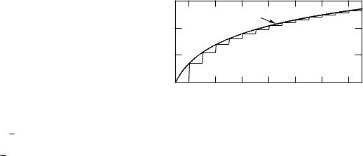
FIGURE I.1. Plot of y = ln m used to derive Stirling’s approximation.
To take the logarithm of Eq. I.1, we need a way to handle the factorials. There is a very useful approximation to the factorial, called Stirling’s approximation:
ln(n!) ≈ n ln n − n. |
(I.2) |
To derive it, write ln(n!) as |
|
|
n |
ln(n!) = ln 1 + ln 2 + · · · + ln n = |
|
ln m. |
|
|
m=1 |
The sum is the same as the total area of the rectangles in Fig. I.1, where the height of each rectangle is ln m and the width of the base is one. The area of all the rectangles is approximately the area under the smooth curve, which is a plot of ln m. The area is approximately
n
ln m dm = [m ln m − m]n1 = n ln n − n + 1.
1
This completes the proof of Eq. (I.2). Table I.1 shows values of n! and Stirling’s approximation for various values of n. The approximation is not too bad for n > 100.