Intermediate Physics for Medicine and Biology - Russell K. Hobbie & Bradley J. Roth

FIGURE 15.23. Calculation of the stopping power at low energies involves integrating the product of the electron charge distribution in the target atom and the interaction strength function, which depends on the projectile speed. The dotted line shows the electron charge density for copper. The solid line shows the integrand. (a) For 10-MeV protons, all electrons but those in the K shell contribute. (b) For 100-keV protons the interaction function has changed, and only the outermost electrons contribute. Note the much di erent ordinate scales in (a) and (b). Provided by J. F. Ziegler.

500 keV. The rise in stopping power at high energies is due to the density e ect (polarization of the electrons).

Another important e ect at low energies is that the slowly moving ion can capture electrons, decreasing the value of z2. Ziegler et al. (1985) discuss the scaling of data for di erent projectiles and the appropriate e ective charge values. The average projectile charge follows a universal curve when plotted as a function of the appropriate combination of the speeds of the projectile and target electrons. They, and the ICRU Report 49 (1993), assume that for protons the e ective charge is always unity. The theoretical justification is that the radius of the electron orbit in hydrogen is larger than the interatomic separation in solids.

15.11.2 Scattering from the Nucleus

The projectile can also scatter from the target atom as a whole. The recoil kinetic energy of the atom is lost by the projectile. Since the nucleus contains most of the mass, the kinematics are those of the bare projectile and the target nucleus, and this process is called nuclear scattering, with stopping power Sn. (Sometimes it is called elastic scattering, with a subscript that can cause it to be confused with electron interactions.)

Just as with Compton scattering, knowing the angle through which the projectile is scattered defines the amount of energy transferred to the target. The angle depends on the impact parameter. The problem can be solved for a given impact parameter if the force between the projectile and target is a function only of their separation and one knows the potential energy of their separation. The details are found in Ziegler et al. (1985). We will simply comment on the contributions to the potential energy. They are

104

Particle energy (eV)

FIGURE 15.24. Proton and electron stopping power vs. energy in carbon, showing the regions in which various models are valid.

1.The Coulomb force between the projectile and the target nucleus.

2.The Coulomb force between the projectile and the electron cloud of the target atom.

3.The Coulomb attraction between the target nucleus and any electrons surrounding the projectile.

4.The Coulomb repulsion between the electron clouds of the target and the projectile.

5.A term due to the Pauli exclusion principle if the projectile is an ion with an electron cloud. To see how it arises, suppose that both the projectile and target have both of their possible K-shell electrons. If the nuclei get close enough, they e ectively form a single nucleus that cannot have four K-shell electrons. Therefore, two of the electrons have to move to unfilled shells. This requires energy that comes from the kinetic energy of the projectile. This is called Pauli promotion. Even though the electrons have time to

return to their original orbits for a slow projectile, the e ect changes the overall potential and hence the projectile orbit and the probability of a particular energy transfer.

6.An exchange term that also arises from the Pauli principle, related to whether the spins of the projectile and target electrons are parallel or antiparallel.

Because nuclear scattering is relatively unimportant for the charged particles we are considering and because it does not lead to ionization, we will not describe any details of the calculations.

15.11.3 Stopping of Electrons

Equations similar to Eq. 15.57 are obtained for electrons and positrons. Recall that energy loss in nuclear scattering is negligible for positrons and electrons because they are so light, and that bremsstrahlung transfers some of the electron kinetic energy to radiation. Electrons and positrons are assumed to collect no screening charge. Even at low energies, the electron velocities are high enough to that the Bethe–Bloch model is used. The collision stopping power for electrons is11

The subscript ± indicates that stopping number per electron is slightly di erent for electrons and for positrons. The exact forms can be found in Attix (1986) or in ICRU Report 37 (1984). In both cases, L depends on I(Z) and the density e ect. An accurate calculation of the shell correction for electrons has not been made; therefore ICRU Report 37 omits the shell correction from the tables for electrons and positrons. This omission makes the use of Eq. 15.59 less accurate for electrons below 10 keV. The best values of Se/ρ for electrons and positrons are obtained from theoretical calculations using Eq. 15.60 and values of I(Z) determined from proton data.

15.11.4Compounds

In dealing with compounds, it is frequently assumed that each atom in the target interacts independently with the projectile, as we assumed for photons. The stopping power per molecule is then equal to the sum of the stopping powers for each atom in the molecule. This leads to a formula analogous to Eq. 15.32, known as the Bragg rule:

This equation applies to the collision, radiative, nuclear, and total stopping powers. This approximation is quite

11The literature often replaces the 4π by 2π for electrons and makes L twice as large.

inaccurate near the peak of the stopping power curve, where the errors can be greater than a factor of 2. This is not surprising, given the behavior of the scattering function I in Fig. 15.23(b). Most of the energy loss is to outer electrons—the conduction electrons if the substance is a metal. In a semiconductor there are gaps in the energy levels, and this precludes the low-energy transfers. As a result, the stopping power is lower in semiconductors. In crystals, channeling can occur: the stopping power depends on the orientation of the trajectory with the crystal symmetry axis.

Carbon poses a particular problem. It is an important element in the body, and it has chemical bonds that range from metallic to insulating in nature. Various investigators have shown variations in stopping power of 30% for ions in pure carbon, depending on how it was fabricated. Graphite can be made with di erent electrical conductivities, and there are associated di erences in stopping power. Ziegler and Manoyan (1988) have applied charge-scaling techniques to several organic carbon compounds by considering separately the stopping due to closed atomic shells (cores) and the remaining bonds between di erent pairs of atoms.

ICRU Reports 37 (1984) and 49 (1993) handle departures from the Bragg rule in the first approximation by using di erent values of I for electrons in compounds. The density e ect is important for electrons and also does not

port 49 has stopping powers for protons and α particles. These data are also found on the web: physics.nist.gov/PhysRefData/Star/Text/contents.html. A computer program for protons and ions, SRIM (Stopping and Range of Ions in Matter) is described by Ziegler et al. (1985) and is available at www.srim.org.

15.12Linear Energy Transfer and Restricted Collision Stopping Power

In modeling the e ect of ionizing radiation on targets, whether they be radiation detectors, photographic emulsions, cells, or parts of cells, one often wants to know how much of a charged particle’s energy is absorbed “locally,” that is, within some region around a particle’s trajectory. An accurate calculation is di cult, since some of the electrons produced may leave the region of interest. Also, the energy absorbed in some region of interest around a particle track comes both from energy lost by the particle while traversing that track segment and also from photons and charged particles produced elsewhere by the projectile. [This is discussed in detail in ICRU Report 16 (1970).]

An approximation to the desired quantity is the linear energy transfer (LET) or the restricted linear collision stopping power L∆. It is defined as the ratio dT /dx, where dx is the distance traveled by the particle and dT is the mean energy loss to electrons that results in energy transfers less than some specified ∆. This use of the symbol L should not be confused with the stopping number of Eqs. 15.57–15.60. The quantity L∆ can be calculated by replacing Wmax by ∆ in the expression for the stopping power. The value of ∆ is usually specified in electron volts.

The electron stopping power Se is numerically equal to L∞. However, Se is defined in terms of the energy lost by the particle, while L∞ is defined in terms of energy imparted to the medium.

Note that although the quantity actually of interest may be the energy imparted within some region around the trajectory, this definition is based on energy transfers less than ∆. A quantity based on the region of interest would be easier to measure; L∆ is easier to calculate.

ICRU Report 37 calculates L∆ for positrons and electrons for values of ∆ down to 1 keV. The report points out that such calculations are inaccurate for smaller values of ∆, even in light elements. ICRU Report 16 provides values of L∆ for protons and heavy ions.

15.13Range, Straggling, and Radiation Yield

We can see in Fig. 15.27 that the α particles, entering from the bottom with the same energy, all travel about the same distance before coming to rest. This distance is called the range of the α particles. It will be defined more precisely below.

We can estimate the range in the following way. The stopping power represents an average energy loss per unit path length. The actual energy loss fluctuates about the mean values given by the stopping power. If these fluctuations are neglected and the projectiles are assumed to lose energy continuously along their tracks at a rate equal to the stopping power, then one is making the continuous- slowing-down approximation (CSDA). In this approximation one can calculate the range, the distance a particle with initial energy T0 travels before coming to rest or reaching some final kinetic energy Tf . A factor ρ is introduced to express the range in mass per unit area:

ICRU Report 37 (1984) discusses the problem of carrying the integration to Tf = 0.

The CSDA range is not directly measurable. Measurements of the fraction F (R) of monoenergetic particles in a beam that passes through an absorber of thickness R

Absorber thickness

FIGURE 15.25. Plot of the number of particles passing through an absorber vs its thickness to show the definition of various ranges. R50 is the median range, Rex is the extrapolated range, and Rm is the maximum range.

gives a curve like that of Fig. 15.25. Various ranges can be defined using this curve. The most easily measured is the median range R50, corresponding to an absorber thickness that transmits 50% of the incident particles. The extrapolated range Rex is obtained by extrapolating the linear portion of the curve to the abscissa. The maximum range Rm is the thickness that just stops all of the particles; it is, of course, very di cult to measure. If F (R) is known accurately one can define a mean range

the transmission curve is perfectly symmetrical about the mean, then R50 is equal to R, even though they are con-

ceptually quite di erent. For heavy projectiles R (usually approximated by R50) provides the best estimate of

RCSDA.

The fluctuations in the range are called straggling. The straggling distribution has also been calculated. The track of a heavy projectile such as an α particle is fairly straight, because the various scattering interactions result only in small angular deviations. The straggling results primarily from the fact that Sdx represents only an average energy loss in path length dx. The fluctuations can be integrated to give the spread in range; see Ahlen (1980) or ICRU Report 37 (1984) or ICRU Report 49 (1993) or the computer program SRIM [Ziegler et al. (1985)].

Electrons and positrons are so light that they undergo large-angle scattering (occasionally from an electron, more often from an atomic nucleus). The resulting electron trajectories are quite tortuous, as can be seen in Figs. 15.28 and 15.29. The median or mean range for an electron is considerably less than RCSDA. For electrons and positrons the extrapolated range Rex corresponds most closely to RCSDA, at least in materials with atomic number up to silver [Tung et al. (1979)]. Figure 15.26 shows ranges in water. At medium energies the dependence on energy is approximately T 2.

Tables of ranges are found in the references cited above or at the NIST web site physics.nist.gov/PhysRefData/Star/Text/contents.html.

Projectile energy (eV)

FIGURE 15.26. Range of electrons, protons, and α particles in liquid water. Data are from ICRU Reports 37 (1984) and 49 (1993). Note that for water the range in gm cm−2 is the same as the range in cm.

The radiation yield, Y , is the fraction of the initial particle (usually electron) kinetic energy T0 that is converted to bremsstrahlung photons as the electron comes to rest in the medium in question. The yield is calculated using the continuous-slowing-down approximation as (neglecting Sn)

15.14 Track Structure

We can gain insight into the interaction processes by examining tracks in photographic emulsions or in cloud chambers. Figures 15.27 and 15.28 are taken from a classic atlas of tracks in nuclear emulsions [Powell et al. (1959)]. They show the di erence between the interaction of heavy and light particles in matter. Figure 15.27 shows the tracks of four cosmic-ray α particles, each of which entered the bottom of the figure and stopped near the top. The fiduciary marks along the bottom are 10 µm apart. Each track is about 195 µm long, corresponding to an initial α-particle energy of about 22 MeV. The emulsion has a density of 3.6 × 103 kg m−3. Each black dot is a sensitive silver halide grain about 0.6 µm in diameter. At the beginning of the track, S is about 70 keV µm−1 or 42 keV per grain; 10 µm from the end of the track it is 200 keV µm−1 or 120 keV per grain. The energy that must be deposited in a grain to render it developable is about 2.8 keV. The amount of energy deposited in each

FIGURE 15.27. Tracks of 22-MeV α particles in photographic emulsion. The α particles enter at the bottom of the page and come to rest near the top. The small square fiducial marks at the bottom are 10 µm apart. The features of the tracks are discussed in the text. From C. F. Powell, P. H. Fowler, and D. H. Perkins. The Study of Elementary Particles by the Photographic Method. Pergamon Press, 1959. Reproduced by permission of Professor D. H. Perkins.

grain is so much larger than this that the track density is uniform. Small bumps of 1–4 grains can be seen occasionally along each track. Some of these are due to δ rays: electrons that have received enough energy to travel a few micrometers in the emulsion. Others are artifacts due to the general background fog. Multiple small-angle scattering causes small deviations in each track, which become greater as the α particle slows down.

In Figure 15.28 an electron–positron pair has been produced in the lower left corner of the emulsion by a 1.5- MeV photon. Each particle has a kinetic energy of about 250 keV. One immediately notices the tortuous path of both particles due to large-angle scattering. The stopping power near the beginning of the track is about 0.8 keV µm−1, so that about 0.5 keV is deposited in each grain. About 30 µm from the end, the stopping power and the average amount of energy deposited in each grain are about 3 times larger. The upper track is considerably more dense near the end of its path. The failure of the other track to show this density increase could be due to annihilation of the positron in flight or to a large-angle scattering out of the emulsion.

FIGURE 15.28. Tracks of electrons in emulsion. An electron— positron pair was produced in the lower left corner. Each particle has an energy of about 250 keV. The details are discussed in the text. From C. F. Powell, P. H. Fowler, and D. H. Perkins. The Study of Elementary Particles by the Photographic Method. Pergamon Press, 1959. Reproduced by permission of Professor D. H. Perkins.

Figure 15.29 shows the ionization produced by an electron at a much di erent scale. It was produced from a cloud chamber photograph of electron tracks in a lowdensity gas [Budd and Marshall (1983)]. The scale shows distances in liquid water or tissue that correspond to the same value of ρx, corrected for phase e ects. Note that the scale shows 10 nanometers. An atomic diameter is 0.2–0.6 nm. In each case a photoelectron of energy between 950 and 1480 eV has been ejected from a gas atom in the cloud chamber. Auger electrons are also seen.

15.15Energy Transferred and Energy Imparted; Kerma and Absorbed Dose

The response of a substance to radiation, whether it is the darkening of a photographic film, an electrical pulse in an ionization chamber, or the response of a tumor to radiation therapy, is due, directly or indirectly, to the ioniza-

FIGURE 15.29. Tracks of ≈1 keV electrons in a cloud chamber. An equivalent scale in water or tissue has been added. Photoelectrons and Auger electrons can be seen. The lines were drawn to guide the eye. From T. Budd and M. Marshall. Microdosimetric properties of electron tracks measured in a low-pressure cloud chamber. Radiation Research 93:19–32 (1983). Reproduced by permission of the Radiation Research Society.

tion produced by charged particles that lose their kinetic energy in the substance through the stopping mechanisms we have just discussed. We now define some quantities that are used to describe the transfer of energy from photons to charged particles and the energy lost by charged particles due to ionization.

15.15.1An Example

Before discussing the formal definition of these quantities, let us consider some examples of energy transfer by photons. Figure 15.30 shows some schematic interactions of photons in a sample of water 10 cm thick. They are drawn to scale.12

In Fig. 15.30(a) five photons of energy 100 keV enter from the left. Photon tracks are dotted. One photon is absorbed by the photoelectric e ect, and four are

12These examples were constructed with a pedagogical simulation program called MacDose [Hobbie (1992)]. The program is available at http://www.oakland.edu/ roth/hobbie.html. It runs on a Macintosh using OS-9 or earlier. A more realistic but easily understood Monte Carlo simulation in described by Arqueros and Montesinos (2003).

Photoelectric Effect

Recoil electron track

(a)

Pair Production

Compton scatter

(b)

FIGURE 15.30. A simulation of photons passing through a layer of water 10 cm thick. (a) The photon energy is 100 keV. One photon has a photoelectric interaction. The other four are Compton scattered. (b) The photon energy is 10 MeV. Two photons do not interact, one produces an electron–positron pair, and two Compton scatter.

Compton scattered. The energy of the photoelectron and the Compton-scattered electrons is so low that the ranges are insignificant on this scale. In Fig. 15.30(b) the incident photons have 10 MeV energy. One has undergone pair production, two have Compton scattered, and two have passed through without interacting. The electron tracks are shown as thick solid lines. Their lengths are equal to the CSDA range of electrons or positrons of that energy. They are drawn as straight lines, even though the real tracks are tortuous.

One of the quantities of interest is the energy transferred to kinetic energy of charged particles in some mass of material. [We saw this briefly in the discussion surrounding Eq. 15.36.] Another is the energy imparted in some mass of material, which is the kinetic energy lost by charged particles as they come to rest. Figure 15.31 shows the distinction between the two quantities. It shows two

3.6

2.00.1

FIGURE 15.31. The di erence between energy transferred and energy imparted. Two of the photons from Fig. 15.30(b) are shown. The water has been divided into ten 1-cm slices. The numbers on the drawing show the charged-particle energy at the entrance to each slice. The energy transferred and the energy imparted in each slice are shown at the bottom.

photons from Fig. 15.30(b): one that underwent pair production, and one that was Compton scattered. The water has been divided into ten slices, each 1 cm thick. No energy is transferred in the first slice. Energy is transferred by pair production in the second slice and by Compton scattering in the third slice. In each case the electron (or positron) produced loses kinetic energy in that slice and also in other slices. There is energy imparted in slices 2– 8, even though the energy is transferred only in slices 2 and 3.

Consider now the actual numbers. In keeping with the literature,13 we will call the energy transferred Etr, even though we have been using T for kinetic energy. For pair production the energy transferred is

Etr = T+ + T− = hν0 − 2mec2

= 10 − 2 × 0.511 = 8.978 ≈ 9.0 MeV. (15.64)

The partition of energy between the electron and positron is stochastic. We assume for this example that about 60% (5.4 MeV) goes to one member of the positron–electron pair and 40% (3.6 MeV) to the other. These numbers are shown at the vertex of Fig. 15.31. From these energies the ranges can be determined. Measuring the distance from the end of the track to the boundary between each slice allows us to determine the energy of each charged particle as it enters the slice. For the Compton scattering, 8.75 MeV is transferred to the recoil electron and the scattered photon has 1.25 MeV. The energy imparted by the 5.4-MeV particle is 5.4 − 4.5 = 0.9 MeV in slice 2,

13See ICRU Report 33 (1980) or Attix (1986).

The quantity R is radiant energy: the energy of particles (including photons) but not including rest energy. The subscript u means that it is the radiant energy of uncharged particles. The uncharged particles can be pho-

14Neutrinos, which we will discuss in Chapter 17, travel such long distances without interacting that they are not considered in the calculations. Energy carried by neutrinos, which come from nuclear β decay, is assumed to have left the body.

15.15.4Net Energy Transferred, Collision Kerma, and Radiative Kerma

Another quantity used in the literature is the net energy transferred. It subtracts from the energy transferred the energy that is reradiated (bremsstrahlung and radiation from positron annihilation in flight), even if the reradiation takes place outside the volume of interest. It is

Etrnet = (Rin)u − (Rout)nonru − Rur + Q. (15.70)

The collision kerma and radiative kerma are defined as expectation values per unit mass:

Considering only a primary beam of monoenergetic photons,

FIGURE 15.33. One of the conditions for charged-particle equilibrium is that on average, for every charged particle of a certain energy leaving volume v traveling in a certain direction, a corresponding particle enters the volume.

value of the energy released by the radioactive material per unit mass. If there is no radioactive source, there is no energy imparted in radiation equilibrium.

15.16 Charged-Particle Equilibrium

There are three equilibrium conditions that sometimes exist or are assumed to exist, that make it possible to calculate the relationship between energy transferred and energy imparted.

15.16.1 Radiation Equilibrium

The first and most restrictive condition is radiation equilibrium. It is a useful model when considering an extended radioactive source that is distributed uniformly throughout some volume V (such as the body or a particular organ). The source is assumed to emit its radiation isotropically. The energy released to neutrinos is ignored. A point of interest within the large volume is surrounded by a smaller volume v. The volume v must be far enough from the edge of V so that any radiation emitted from v is absorbed before reaching the surface of V . The entire volume V is assumed to be of the same atomic composition and density. Because everything is isotropic, on average for every photon or neutron or charged particle entering volume v, another identical one leaves. This means that

The average energy imparted is

E = Q. (15.74)

This means that when the conditions for radiation equilibrium are satisfied, the absorbed dose is the expectation

15.16.2Charged-particle Equilibrium

A less restrictive assumption is charged-particle equilibrium, in which only Eq. 15.73a is satisfied: the average amount of charged-particle radiant energy entering the region is the same as the average amount leaving. The assumption of charged particle equilibrium is a useful model in several cases, but we will consider only the case of an external beam of photons striking volume V . Again we consider what happens in a smaller volume v, separated from the boundary of V by a distance larger than the maximum range of any secondary charged particles produced by the external radiation. We also assume that the medium is homogeneous and that only a small fraction of the primary radiation interacts within the volume so attenuation can be neglected. Then the average number of charged particles produced per unit volume and per unit solid angle in any given direction is the same everywhere in the volume. Though the charged particles need not be produced isotropically, on average for every particle that leaves volume v, a corresponding one will enter it, as shown in Fig. 15.33. For charged-particle equilibrium, the average energy imparted is

E = Rin u − Rout u + Q.

Comparing this with the average of Eq. 15.70 shows that the average net energy transferred is

Etrnet = E + Rout u − Rout

the average value of all uncharged radiation leaving excluding bremsstrahlung and photons from annihilation

in flight that occur within the volume, and Rur is the bremsstrahlung and annihilation-in-flight radiation from charged particles originating in v regardless of where it occurs. If there is charged-particle equilibrium, any radiative interaction by a charged particle after it leaves the volume will on average be replaced by an identical interaction inside v. If the volume is small enough so that all radiative loss photons escape from the volume before undergoing any subsequent interactions, then

Therefore, for charged-particle equilibrium, E = Etrnet, and the dose is equal to the collision kerma:

One situation where charged-particle equilibrium applies is for the thin slices in Fig. 15.30(a). The electron ranges are so short (10 µm for a 25-keV electron) that a slice can be thin compared to 1/µ and yet all the electrons produced stay within the volume.

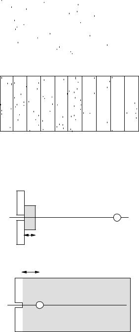
The conditions for charged-particle equilibrium fail if the source of photons is too close (Ψ is not uniform because of 1/r2), close to a boundary (as between air and tissue or muscle and bone), for high-energy radiation (as in Fig. 15.32), or if there is an applied electric or magnetic field that alters the paths of the charged particles (as in some radiation detectors).

In Fig. 15.32, if we look at the situation far enough to the right, the energy imparted is proportional to the energy transferred. This situation is called transient charged-particle equilibrium.

The dose for a monoenergetic parallel beam of charged particles with particle fluence Φ passing through a thin layer can be calculated by making three assumptions:

1.The volume of interest is thin enough so that Se remains constant.

2.Scattering can be neglected, so every particle passes straight through the layer.

3.The net kinetic energy carried out of the layer by δ rays is negligible, either because the layer is thick compared to the range of the δ rays or because the layer is immersed in a material of the same atomic number so that charged-particle equilibrium exists.

Then the energy lost in collisions in a layer of thickness dz is E = Φ(area)(Se/ρ)ρdz and the mass is ρ(area)dz, so the dose is

Attix (1986, pp. 188–195) discusses corrections for situations where these assumptions are not valid.

(b)

FIGURE 15.34. Secondary photons also interact in this simulation. One 100-keV photon enters from the left in each panel.

(a) The primary photon undergoes a Compton scattering. The Compton-scattered photon also undergoes a Compton scattering. The third photon escapes from the water. (b) The primary photon is Compton scattered. Each Compton-scattered photon undergoes another Compton scattering, until the sixth scattered photon leaves through the upstream surface of the water, traveling nearly in the direction from which the incident photon came.

15.17 Buildup

We have been ignoring the interactions of secondary photons, primarily Compton-scattered photons and annihilation radiation. They can be quite significant. In fact, there can be a cascade of several generations of photons, though we will call them all “secondary photons.” Figure 15.34 compares two simulations in which the secondary photons are allowed to interact. In Fig. 15.34(a) there is one secondary interaction before the scattered photon escapes from the water. In Fig. 15.34(b) there are a total of six Compton scatterings before the secondary photon escapes.

All of these secondary photons produce electrons that contribute to the energy transferred and energy imparted. Figure 15.35 compares two cases where 25 photons of energy 100 keV enter the water from the left. The primary interactions are the same in both cases. In Fig. 15.35(a) the small dots represent the electrons produced by the interaction of the primary photons. In Fig. 15.35(b) the electrons produced by secondary and subsequent interactions are also shown. The energy transferred and energy imparted are much greater.

The buildup factor for any quantity is defined as the ratio of the quantity including secondary and scattered radiation to the quantity for primary radiation only. For example, if the primary beam has an energy fluence Ψ0 at the surface, the energy fluence at depth x in

Symbols Used in Chapter 15

the medium is

The buildup factor is quite sensitive to the geometry. Compare the two situations in Fig. 15.36. In Fig. 15.36(a) the detector is at a fixed location and the thickness of

wi

x, y, z x

z

A