Intermediate Physics for Medicine and Biology - Russell K. Hobbie & Bradley J. Roth

An x-ray image records variations in the passage of x rays through the body because of scattering and absorption. A side e ect of making the image is the absorption of some x-ray energy by the body. Radiation therapy depends on the absorption of large amounts of x-ray energy by a tumor. Diagnostic procedures in nuclear medicine (Chapter 17) introduce a small amount of radioactive substance in the body. Radiation from the radioactive nuclei is then detected. Some of the energy from the photons or charged particles emitted by the radioactive nucleus is absorbed in the body. To describe all of these e ects requires that we understand the interaction of photons and charged particles with matter.

In Chapter 14 we discussed the transport of photons of ultraviolet and lower energy—a few electron volts or less. Now we will discuss the transport of photons of much higher energy—10 keV and above. We will also discuss the movement through matter of charged particles such as electrons, protons, and heavier ions. These high energy photons and charged particles are called ionizing radiation, because they produce ionization in the material through which they pass. The distinction is blurred, since ultraviolet light can also ionize.

A charged particle moving through matter loses energy by local ionization, disruption of chemical bonds, and increasing the energy of atoms it passes near. It is said to be directly ionizing. Photons passing through matter transfer energy to charged particles, which in turn a ect the material. These photons are indirectly ionizing.

Photons and charged particles interact primarily with the electrons in atoms. Section 15.1 describes the energy levels of atomic electrons. Section 15.2 describes the various processes by which photons interact; these are elaborated in the next four sections, leading in Sec. 15.7 to the concept of a photon attenuation coe cient.

Attenuation is extended to compounds and mixtures in Sec. 15.8.

An atom is often left in an excited state by a photon interaction. The mechanisms by which it loses energy are covered in Sec. 15.9. The energy that is transferred to electrons can cause radiation damage. The transfer process is described in Secs. 15.10 and 15.15–15.17.

Section 15.11 introduces the charged-particle stopping power, which is the rate of energy loss by a charged particle as it passes through material. Extensions of this concept, which are important in radiation damage, are the linear energy transfer and the restricted collision stopping power, introduced in Sec. 15.12. A charged particle travels a certain distance through material as it loses its kinetic energy. This leads in Sec. 15.13 to the concept of range. Charged particles also lose energy by emitting photons. The radiation yield is also discussed in Sec. 15.13. Insight into the process of radiation damage is gained by examining track structure in Sec. 15.14.

The last three sections return to the movement of energy from a photon beam to matter. The discussion requires an understanding of both photon interactions and charged-particle stopping power and range.

15.1Atomic Energy Levels and X-ray Absorption

A neutral atom has a nuclear charge +Ze surrounded by a cloud of Z electrons. As was described in Chapter 14, each electron has a definite energy, characterized by a set of five quantum numbers: n, l, s (which is always 12 ), j, and mj . (Instead of j and mj , the numbers ml and ms

TABLE 15.1. Energy levels for electrons in a tungsten atom (Z = 74)

are sometimes used.) There are restrictions on the values of the numbers:

The dependence of the electron energy on mj is very slight, unless the atom is in a magnetic field.

In each atom, only one electron can have a particular set of values of the quantum numbers. Since the atoms we are considering are not in a magnetic field, electrons with di erent values of mj but the same values for n, l, and j will all be assumed to have the same energy. Electrons with di erent values of n are said to be in di erent shells. The shell for n = 1 is called the K shell; those for n = 2, 3, 4, . . . are labeled L, M, N, . . . . Di erent values

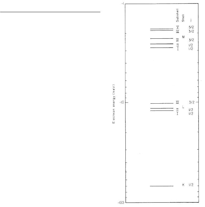
FIGURE 15.1. Energy levels for electrons in tungsten.

of l and j for a fixed value of n are called subshells, denoted by roman numeral subscripts on the shell labels. The maximum number of electrons that can be placed in a subshell is 2(2l + 1). Each electron bound to the atom has a certain negative energy, with zero energy defined when the electron is just unbound, that is, at rest infinitely far away from the atom. Table 15.1 lists the energy levels of electrons in tungsten. Some of the levels in Table 15.1 are shown in Fig. 15.1. The scale is logarithmic. Since the energies are negative, the magnitude increases in the downward direction. Tables of atomic energy levels can be

found many places, including www.csrri.iit.edu/periodictable.html.

The ionization energy is the energy required to remove the least-tightly-bound electron from the atom. For tungsten, it is about 6 eV. If one plots the ionization energy or the chemical valence of atoms as a function of Z, one finds abrupt changes when the last electron’s value of n or l changes.

In contrast to this behavior of the outer electrons, the energy of an inner electron with fixed values of n and l varies smoothly with Z. To a first approximation, the two innermost K electrons are attracted to the nuclear charge Ze. The energy of the level can be estimated using Eq. 14.8 for hydrogen, with the nuclear charge e replaced by

Ze:

The two electrons also repel each other and experience some repulsion by electrons in other shells. This e ect is called charge screening. Experiment (measuring values of EK ) shows that the e ective charge seen by a K electron is approximately Ze ≈ Z −3 for heavy elements, so that for K electrons (n = 1),

The screening is greater for electrons with larger values of n, which may be thought of as being in “orbits” of larger radius.

15.2 Photon Interactions

There are a number of di erent ways in which a photon can interact with an atom. The more important ones will be considered here. It is convenient to adopt a notation (γ, bc) where γ represents the incident photon and b and c are the results of the interaction. For example, (γ, γ) represents initial and final photons having the same energy; in a (γ, e) interaction the photon is absorbed and only an electron emerges. This section describes the common interactions and the energy balance for each case.

15.2.1 Photoelectric E ect

In the photoelectric e ect, (γ, e), the photon is absorbed by the atom and a single electron is ejected. The initial photon energy hν0 is equal to the final energy. The recoil kinetic energy of the atom is very small because its mass is large, so the final energy is the kinetic energy of the electron, Tel, plus the excitation energy of the atom. The excitation energy is equal to the binding energy of the ejected electron, B. The energy balance is therefore

The atom subsequently loses its excitation energy. The deexcitation process described in Sec. 15.9 involves the

emission of additional photons or electrons. The photoelectric cross section is τ .

15.2.2Compton and Incoherent Scattering

In Compton scattering, (γ, γ e), the original photon disappears and a photon of lower energy and an electron emerge. The statement of energy conservation is

hν0 = hν + Tel + B.

Usually the photon energy is high enough so that B can be neglected, and this is written as

The Compton cross section for scattering from a single electron is σC . Incoherent scattering is Compton scattering from all the electrons in the atom, with cross section

σincoh.

15.2.3Coherent Scattering

Coherent scattering is a (γ, γ) process in which the photon is elastically scattered from the entire atom. That is, the internal energy of the atom does not change. The recoil kinetic energy of the atom is very small (see Problem 6), and it is a good approximation to say that the energy of the incident photon equals the energy of the scattered photon:

The cross section for coherent scattering is σcoh.

15.2.4Inelastic Scattering

It is also possible for the final photon to have a di erent energy from the initial photon (γ, γ ) without the emission of an electron. The internal energy of the target atom or molecule increases or decreases by a corresponding amount. Again, the recoil kinetic energy of the atom is negligible. Examples are fluorescence and Raman scattering. In fluorescence, if one waits long enough, additional

photons are emitted, in which case the reaction could be denoted as (γ, γ γ ), or (γ, 2γ), or even (γ, 3γ).

15.2.5Pair Production

Pair production takes place at high energies. This is a (γ, e+e−) reaction. Since it takes energy to create the (negative) electron and the positive electron or positron, their rest energies must be included in the energy balance equation:

hν0 = T+ +mec2 +T− +mec2 = T+ +T− +2mec2. (15.7)

The cross section for pair production is κ.

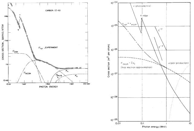
FIGURE 15.2. Total cross section for the interactions of photons with carbon vs. photon energy. The photoelectric cross section is τ , the coherent scattering cross section σcoh, the total Compton cross section σincoh, and the nuclear and electronic (triplet) pair production are κn and κe. The photonuclear scattering cross section PHN is also shown. The cross section is given in barns: 1 b = 10−28 m2. Reprinted with permission from J. H. Hubbell, H. A. Gimm, and I. Øverbø (1980). Pair, triplet and total atomic cross sections (and mass attenuation coe cients) for 1 MeV–100 GeV photons in elements Z = 1 to 100. J. Phys. Chem. Ref. Data 9: 1023–1147. Copyright 1980, American Institute of Physics. Figure courtesy of J. H. Hubbell.

15.2.6 Energy Dependence

Figure 15.2 shows the cross section for interactions of photons with carbon for photon energies from 10 to 1011 eV. At the lowest energies the photoelectric e ect dominates. Between 10 keV and 10 MeV Compton scattering is most important. Above 10 MeV pair production takes over. There is a small bump at about 20 MeV due to nuclear e ects, but its contribution to the cross section is only a few percent of that due to pair production. The four important e ects are discussed in the next four sections.

15.3 The Photoelectric E ect

In the photoelectric e ect a photon of energy hν0 is absorbed by an atom, and an electron of kinetic energy Tel = hν0 − B is ejected. B is the magnitude of the binding energy of the electron and depends on which shell the electron was in. Therefore it is labeled BK , BL, and so forth. The cross section for the photoelectric e ect, τ , is a sum of terms for each shell:

FIGURE 15.3. Cross sections for the photoelectric e ect and incoherent and coherent scattering from lead. The binding energies of the K and L shells are 0.088 and 0.0152 MeV. Plotted from Table 3.22 of Hubbell (1969).

As the energy of a photon beam is decreased, the photoelectric cross section increases rapidly. For photon energies too small to remove an electron from the K shell, the cross section for the K-shell photoelectric e ect is zero. Even though photons do not have enough energy to remove an electron from the K shell, they may have enough energy to remove L-shell electrons. The cross section for L electron photoelectric e ect is much smaller than that for K electrons, but it increases with decreasing energy until its threshold energy is reached. This energy dependence is shown for lead in Fig. 15.3, which plots the cross section for the photoelectric e ect, incoherent Compton scattering, and coherent scattering. The K absorption edge for the photoelectric e ect is seen. The photoelectric e ect below the K absorption edge is due to L, M, . . . electrons; above this energy the K electrons also participate. Above 0.8 MeV in lead Compton scattering becomes more important than the photoelectric e ect.

The energy dependence of the photoelectric e ect cross section is between E−2 and E−4. An approximation to the Z and E dependence of the photoelectric cross section near 100 keV is

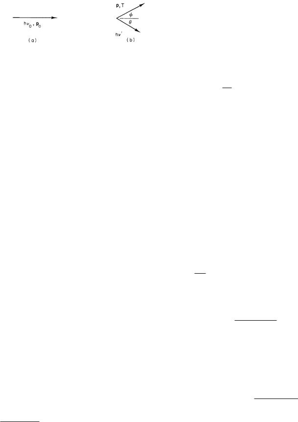
FIGURE 15.4. Momentum relationships in Compton scattering. (a) Before. (b) After. The photon emerges at angle θ, the electron at angle φ.

Once an atom has absorbed a photon and ejected a photoelectron, it is in an excited state. The atom will eventually lose this excitation energy by capturing an electron and returning to its ground state. The deexcitation processes are described in Sec. 15.9.

15.4 Compton Scattering

15.4.1 Kinematics

Compton scattering is a (γ, γ e) process. The equations that are used to relate the energy and angle of the emerging photon and electron, as well as the equations that give the cross section for the scattering, are usually derived assuming that the electron is free and at rest. We turn first to the kinematics. A photon has energy E and momentum p, related by

This is a special case of a more general relationship from special relativity:

In these equations E is the total energy of the particle, p its momentum, m0 the “rest mass” of the particle (measured when it is not moving), and m0c2 is the “rest energy.”1 For a photon, which can never be at rest, m0 = 0. Equation 15.10 can also be derived from the classical electromagnetic theory of light.

The conservation of energy and momentum can be used to derive the relationship between the angle at which the scattered photon emerges and its energy. A detailed knowledge of the forces involved is necessary to calculate the relative number of photons scattered at di erent angles; in fact, this calculation must be done using quantum mechanics. Figure 15.4 shows the geometry involved in the scattering. The electron emerges with momentum p, kinetic energy T , and total energy E = T + mec2. It emerges at an angle φ with the direction of the incident photon. The scattered photon emerges at angle θ with a

1Since this is one of the few relativistic results we will need, it is not developed here. A discussion can be found in any book on special relativity.

reduced energy and a corresponding frequency ν which is lower than ν0, the frequency of the incident photon. Conservation of momentum in the direction of the incident photon gives

while conservation of momentum at right angles to that direction gives

hνc sin θ = p sin φ.

Conservation of energy gives

hν0 = hν + T.

The equation E = T + mec2 can be combined with Eq. 15.11 to give

(pc)2 = T 2 + 2mec2T.

The last four equations can then be combined and solved for various unknowns.

The wavelength of the scattered photon is

The wavelength shift (but not the frequency or energy shift) is independent of the incident wavelength. The quantity h/mec has the dimensions of length and is called the Compton wavelength of the electron. Its numerical value is

If Eq. 15.12 is solved for the energy of the scattered photon, the result is

where x is the energy of the incident photon in units of mec2 = 511 keV:

The energy of the recoil electron is T = hν0 − hν :

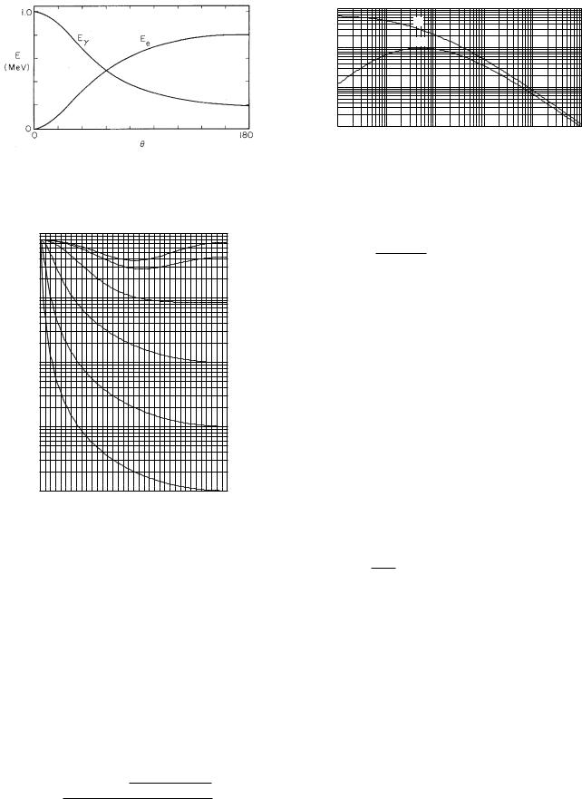
Figure 15.5 shows the energy of the scattered photon and the recoil electron as a function of θ, the angle of emergence of the photon. The sum of the two energies is 1 MeV, the energy of the incident photon.

FIGURE 15.5. The energy of the emerging photon and recoil electron as a function of θ, the angle of the emerging photon, for a 1-MeV incident photon.

Incident photon energy (MeV)

FIGURE 15.7. The total cross section σC for Compton scattering by a single electron and the cross section for energy transfer σtr = fC σC .

where

is the “classical radius” of the electron. The cross section is plotted in Fig. 15.6. It is peaked in the forward direction at high energies. As x → 0 (long wavelengths or low energy) it approaches

which is symmetric about 90 ◦.

Equation 15.17 can be integrated over all angles to obtain the total Compton cross section for a single electron:

FIGURE 15.6. Di erential cross section for Compton scattering of unpolarized photons from a free electron, calculated from Eq. 15.17. The incident photon energy for each curve is shown on the right.

15.4.2 Cross Section: Klein–Nishina Formula

The inclusion of dynamics, which allows us to determine the relative number of photons scattered at each angle, is fairly complicated. The quantum-mechanical result is known as the Klein–Nishina formula. The result depends on the polarization of the photons. For unpolarized photons, the cross section per unit solid angle for a photon to be scattered at angle θ is

Figure 15.7 shows σC as a function of energy.

The classical analog of Compton scattering is Thomson scattering of an electromagnetic wave by a free electron. The electron experiences the electric field E of an incident plane electromagnetic wave and therefore has an acceleration −eE/m. Accelerated charges radiate electromagnetic waves, and the energy radiated in di erent directions can be calculated, giving Eqs. 15.18 and 15.20. [See, for example, Rossi (1957, Chapter 8).] In the classical limit of low photon energies and momenta, the energy of the recoil electron is negligible.

the incoherent cross section occurs if all Z electrons take part in the Compton scattering:

σincoh ≤ ZσC .

For carbon ZσC = 4.0 × 10−28 m2. This value is approached by σincoh near 10 keV. At low energies σincoh falls below this maximum value because the electrons are bound and not at rest. This fallo can be seen in Fig. 15.2. It is appreciable for energies as high as 7–8 keV, even though the K-shell binding energy in carbon is only 283 eV. The electron motion and binding in the target atom also cause a small spread in the energy of the scattered photons [Carlsson et al. (1982)].

Departures of the angular distribution and incoherent cross section from Z times the Klein–Nishina formula are discussed by Hubbell et al. (1975) and by Jackson and Hawkes (1981).

15.4.4 Energy Transferred to the Electron

We will need to know the average energy transferred to an electron in a Compton scattering. Equation 15.16 gives the electron kinetic energy as a function of photon scattering angle. The transfer cross section is defined to be

This can be integrated. The result is [see Attix (1986), p. 134]

This quantity is also plotted in Fig. 15.7. Equation 15.22 is a rather nasty equation to evaluate, particularly at low energies, because many of the terms nearly cancel.

15.5 Coherent Scattering

A photon can also scatter elastically from an atom, with none of the electrons leaving their energy levels. This (γ, γ) process is called coherent scattering (sometimes called Rayleigh scattering), and its cross section is σcoh. The entire atom recoils; if one substitutes the atomic mass in Eqs. 15.15 and 15.16, one finds that the atomic recoil kinetic energy is negligible.

The primary mechanism for coherent scattering is the oscillation of the electron cloud in the atom in response to the electric field of the incident photons. There are small contributions to the scattering from nuclear processes.

The cross section can be calculated classically as an extension of Thomson scattering, or it can be done using various degrees of quantum-mechanical sophistication [see Kissel et al. (1980) or Pratt (1982)].

The coherent cross section is peaked in the forward direction because of interference e ects between electromagnetic waves scattered by various parts of the electron cloud. The peak is narrower for elements of lower atomic number and for higher energies. Coherent and incoherent scattering cross sections are shown in Fig. 15.8 for 100keV photons scattering from carbon, calcium, and lead. Also shown for comparison is Z(dσ/dΩ)KN .

If the wavelength of the incident photon is large compared to the size of the atom, then all Z electrons behave like a single particle with charge −Ze and mass Zme. From Eqs. 15.18 and 15.20, one can see that the cross section in this limit is Z2 times the single-electron value: Z2σC . The limiting value for carbon is 2.39 × 10−27 m2, which can be compared to the low energy limit for σcoh in Fig. 15.2.

15.6 Pair Production

A photon with energy above 1.02 MeV can produce a particle–antiparticle pair: a negative electron and a positive electron or positron. Conservation of energy requires that

electron positron

(15.23) Since the rest energy (mec2) of an electron or positron is 0.51 MeV, pair production is energetically impossible for photons below 2mec2 = 1.02 MeV.

One can show, using hν0 = pc for the photon, that momentum is not conserved by the positron and electron if Eq. 15.23 is satisfied. However, pair production always takes place in the Coulomb field of another particle (usually a nucleus) that recoils to conserve momentum. The nucleus has a large mass, so its kinetic energy p2/2m is small compared to the terms in Eq. 15.23. The cross section for this (γ, e+e−) reaction involving the nucleus is

κn.

Pair production with excitation or ionization of the recoil atom can take place at energies that are only slightly higher than the threshold; however, the cross section does not become appreciable until the incident photon energy exceeds 4mec2 = 2.04 MeV, the threshold for pair production in which a free electron (rather than a nucleus) recoils to conserve momentum. Because ionization and free-electron pair production are (γ, e−e−e+) processes, this is usually called triplet production. Extensive data are given in Hubbell et al. (1980).

The cross section for both processes is κ = κn + κe. The energy dependence of κ can be seen in Figs. 15.2 and 15.3.

FIGURE 15.9. Measurements with (a) narrow-beam geometry and (b) broad-beam geometry.

15.7The Photon Attenuation Coe cient

Consider the arrangement shown in Fig. 15.9(a), in which a beam of photons is collimated so that a narrow beam strikes a detector.

A scattering material is then introduced in the beam. Some of the photons pass through the material without interaction. Others are scattered. Still others disappear because of photoelectric e ect or pair-production interactions. If we measure only photons that remain in the unscattered beam, the loss of photons is called attenuation of the beam. Attenuation includes both scattering and absorption. We record as still belonging to the beam only photons that did not interact; they still travel in the forward direction with the original energy. This is called a narrow-beam geometry measurement. It is an idealization, because photons that undergo Compton or coherent scattering through a small angle can still strike the detector. Figure 15.9(b) shows a source, scatterer, and detector geometry that is much more di cult to interpret. In this case photons that are initially traveling in a di erent direction are scattered into the detector. These are called broad-beam geometry experiments.

In narrow-beam geometry, the total cross section is related to the total number of particles that have interacted in the scatterer. Let N be the number of particles that have not undergone any interaction in passing through scattering material of thickness z. We saw in Sec. 14.4 that the number of particles that have not interacted decreases in thickness dz by

dN = −σtotNAρ N dz, A

In these equations ρ is the mass density of the target material and A is its atomic weight.2 The number of particles that have undergone no interaction decays exponentially with distance:

The quantity µatten is called the total linear attenuation coe cient.

In a broad-beam geometry configuration the total number of photons reaching the detector includes secondary photons and is larger than the value given by Eq. 15.25.

The units in Eqs. 15.24 and 15.25 are worth discussing. Avogadro’s number is 6.022 045 × 1023 entities mol−1. If the density ρ is in kg m−3 and σtot is in m2, then A must be expressed in kg mol−1 and µatten is in m−1. On the other hand, it is possible to express ρ in g cm−3, σtot in cm2, and A in g mol−1, so that µatten is in cm−1. As an example, consider carbon, for which A = 12.011 × 10−3

kg mol−1 = 12.011 g mol−1. If σtot = 1.269 × 10−28 m2 atom−1 = 1.269 × 10−24 cm2 atom−1, then either

FIGURE 15.10. Mass attenuation coe cient vs. energy for lead, calcium, and water. Near 1 MeV the mass attenuation coe cient is nearly independent of Z. Plotted from data provided by NIST: http://physics.nist.gov/PhysRefData/Xcom /Text/XCOM.html.

(6.022 × 1023 atom mol−1)(2.000 × 103 kg m−3) µatten = 12.011 × 10−3 kg mol−1

× (1.269 × 10−28 m2 atom−1) = 12.7 m−1

or

In many situations the coherently scattered photons cannot be distinguished from those unscattered, and σcoh should not be included:

Tables usually include total cross sections and attenuation coe cients both with and without coherent scattering.

It is possible to regroup the terms in Eqs. 15.24 and 15.25 in a slightly di erent way:

dN = −N NAσtot ρdz. A

2The atomic weight is potentially confusing. Sometimes A has no units (as in labeling an nuclear isotope), sometimes it is in grams per mole, and sometimes it is in kilograms per mole).

The quantity NAσtot/A is the mass attenuation coe - cient, µatten/ρ (m2 kg−1):

The exponential attenuation is then

The mass attenuation coe cient has the advantage of being independent of the density of the target material, which is particularly useful if the target is a gas. It has an additional advantage if Compton scattering is the dominant interaction. If σtot = ZσC , then

µatten = ZσC NA .

ρ A

Since Z/A is nearly 1/2 for all elements except hydrogen, this quantity changes very little throughout the periodic table. This constancy is not true for the photoelectric e ect or pair production. Figure 15.10 plots the mass attenuation coe cient vs energy for three elements spanning the Periodic Table. It is nearly independent of Z around 1 MeV where Compton scattering is dominant. The K and L absorption edges can be seen for lead; for the lighter elements they are below 10 keV.

Figure 15.11 shows the contributions to µatten/ρ for air from the photoelectric e ect, incoherent scattering, and pair production. Tables of mass attenuation coe cients

Photon energy (MeV)

FIGURE 15.11. Mass attenuation coe cient vs energy for air. Plotted from data provided by NIST: http://physics.nist.gov /PhysRefData/Xcom/Text/XCOM.html.

are provided by the National Institute of Standards and Technology (NIST) at physics.nist.gov/PhysRefData/.

The mass fraction of element i in a compound containing ai atoms per molecule with atomic mass Ai is

The factor (NT V )mol = ρNA/Amol is the number of molecules per unit volume. When a target entity (molecule) consists of a collection of subentities (atoms), we can say that in this approximation (all subentities interacting independently), the cross section per entity is the sum of the cross sections for each subentity. For example, for the molecule CH4, the total molecular cross section is σcarbon + 4σhydrogen and the molecular weight is [(4 × 1) + 12 = 16] × 10−3 kg mol−1.

15.8 Compounds and Mixtures

The usual procedure for dealing with mixtures and compounds is to assume that each atom scatters independently. If the cross section for element i summed over all the interaction processes of interest is denoted by σi, then Eq. 14.18 is replaced by

where (NT )i is the number of target atoms of species i per unit projected area of the target and (NT V )i is the number of target atoms per unit volume. The sum is taken over all elements in the compound or mixture.

It is possible to replace the sum by the product of the cross section per molecule multiplied by the number of molecules per unit volume. The cross section per molecule is the sum of the cross sections for all the atoms in the molecule. To see that this is so, note that a volume of scatterer V contains a total mass M = ρV. The mass of each element is Mi and the mass fraction is wi = Mi/M . The total number of atoms of species i in volume V is the number of moles times Avogadro’s number:

15.9 Deexcitation of Atoms

After the photoelectric e ect, Compton scattering, or triplet production, an atom is left with a hole in some electron shell. An atom can be left in a similar state when an electron is knocked out by a passing charged particle or by certain transformations in the atomic nucleus that are discussed in Chapter 17.

The hole in the shell can be filled by two competing processes: a radiative transition, in which a photon is emitted as an electron falls into the hole from a higher level, or a nonradiative or radiationless transition, such as the emission of an Auger electron from a higher level as a second electron falls from a higher level to fill the hole. Both processes are shown in Fig. 15.12. In the radiative transition, the energy of the photon is equal to the di erence in binding energies of the two levels. For the example of Fig. 15.12(b), the photon energy is BK − BL. The emission of an L-shell Auger electron is shown in Fig. 15.12(c): its energy is T = (BK −BL) −BL = BK −2BL. Table 15.2 shows the energy changes that occur after a hole is created in an atom by photoelectric excitation. It is worth understanding each table entry in detail. Two di erent paths for deexcitation are shown: one for photon emission and one for ejection of an Auger electron. The sum of the photon, electron, and atomic excitation energies does not change.

The photon that is emitted is called a characteristic photon or a fluorescence photon. Its energy is given by the di erence of two electron energy levels in the atom. There is an historical nomenclature for these photons.