Intermediate Physics for Medicine and Biology - Russell K. Hobbie & Bradley J. Roth

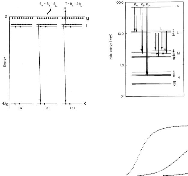
Because a hole moving to larger values of n corresponds to a decrease in the total energy of an atom, it is customary to draw the energy levels for holes instead of electrons, as in Fig. 15.13. Transitions in which the hole is initially in the n = 1 state give rise to the K series of x rays, those in which the initial hole is in the n = 2 state give rise to the L series, and so on. Greek letters (and their subscripts) are used to denote the shell (and subshell) of the final hole. The transitions shown in Fig. 15.13 are consistent with certain selection rules which can be derived using quantum theory:

We saw in Eqs. 15.2 and 15.3 that the position of a level could be estimated by the Bohr formula corrected for screening. The energy of the Kα line—which depends on screening for both the initial (n = 2) and final (n = 1) values of n—can be fitted empirically by

After creation of a hole in the K shell, it is random whether the atom deexcites by emitting a photon or an Auger electron. The probability of photon emission is called the fluorescence yield, WK . The Auger yield is AK = 1 − WK . For a vacancy in the L or higher shells, one must consider the fluorescence yield for each subshell, defined as the number of photons emitted with an initial

state corresponding to a hole in a subshell, divided by the number of holes in that subshell. The situation is further complicated by the fact that radiationless transitions can take place within the subshell, thereby altering the number of vacancies in each subshell. These are called

Coster–Kronig transitions, and they are also accompanied by the emission of an electron. For example, a hole in the LI shell can be filled by an electron from the LIII shell with the ejection of an M -shell electron. A super- Coster–Kronig transition involves electrons all within the same shell, for example, a hole in the MI shell filled by an electron from the MII shell with the ejection of an electron from the MIV shell.

One can define an average fluorescence yield W L, W M , etc. for each shell, but it is not a fundamental property of the atom, since it depends on the vacancy distribution in the subshells. Bambynek et al. (1972) review the physics of atomic deexcitations and present theoretical and experimental data for the fundamental parameters. They show that W L is less sensitive to the initial vacancy distribution than one might expect, because of the rapid changes in hole distribution caused by the Coster–Kronig transitions. Hubbell et al. (1994) provide a more recent review. Figure 15.14 shows values for WK , W L, and W M as a function of Z. One can see from this figure that radiationless transitions are much more important (the fluorescent yield is much smaller) for the L shell than for the K shell. They are nearly the sole process for higher shells. The deexcitation is often called the Auger cascade.

FIGURE 15.12. Two possible mechanisms for the deexcitation of an atom with a hole in the K shell. (a) The atom with the hole in the K shell. (b) An electron has moved from the L shell to the K shell with emission of a photon of energy BK − BL.

(c) An electron has moved from the L shell to the K shell. The energy liberated is taken by another electron from the L shell, which emerges with energy BK − 2BL. This electron is called an Auger electron.

The Auger cascade produces many vacancies in the outer shells of the atom, and some of these may be filled by electrons from other atoms in the same molecule. This process can break molecular bonds. Moreover, the Auger and Coster–Kronig electrons from the higher shells can be quite numerous. They are of such low energy that they travel only a fraction of a cell diameter. This must be taken into consideration when estimating cell damage from radiation. The e ect of radiationless transitions is quite important for certain radioactive isotopes that are administered to a patient, particularly when they are bound to the cellular DNA. We will discuss them further in Chapter 17.

15.10Energy Transfer from Photons to Electrons

The attenuation coe cient gives the rate at which photons interact and leave the primary beam as they pass through material. If a beam of monoenergetic photons of energy E = hν and particle fluence Φ passes through a thin layer dx of material, the number of particles

FIGURE 15.13. Energy-level diagram for holes in tungsten, and some of the x-ray transitions.

Z

FIGURE 15.14. Fluorescence yields for K-, L-, and M -shell vacancies as a function of atomic number Z. Points are from Table 8 of Hubbell et al. (1994).

per unit area that interact in the layer, −dΦ, is proportional to the fluence and the attenuation coe cient: −dΦ = Φµatten dx. The energy fluence is Ψ = hνΦ. The reduction of energy fluence of unscattered photons is −dΨ = −hν dΦ. For a thick absorber we can say that the number of unscattered photons and the energy carried by unscattered photons decay as

Φunscatt = Φ0e−µattenx, Ψunscatt = Ψ0e−µattenx.

(15.35)

The total energy flow is much more complicated. Every photon that interacts contributes to a pool of secondary

FIGURE 15.15. Routes for the transfer of energy between photons and electrons.

photons of lower energy and to a pool of electrons and positrons. Figure 15.15 shows the processes by which energy can move between the photon pool and the electron– positron pool. Energy that remains as secondary photons, such as those resulting from fluorescence or Compton scattering, can travel long distances from the site of the initial interaction. Ionizing particles (photoelectrons, Auger electrons, Compton recoil electrons, and electron– positron pairs) usually lose their energy relatively close to where they were produced. We will see in Sec. 15.13 that for primary photons below 10 MeV, the mean free path of the secondary electrons is usually short compared to that of the photons. Damage to cells is caused by local ionization or excitation of atoms and molecules. This damage is done much more e ciently by the electrons than by the photons.

The mass energy transfer coe cient µtr/ρ is a measure of the energy transferred from primary photons to charged particles in the interaction. If N monoenergetic photons of energy E strike a thin absorber of thickness dx, the amount of energy transferred to charged particles is defined to be

We can relate µtr to µatten. Suppose the material contains a single atomic species and that fi is the average fraction of the photon energy that is transferred to charged particles in process i. (Di erent values of i denote the photoelectric e ect, incoherent scattering, coherent scattering, and pair production.) Multiplying the number of photons that interact by their energy E and by fi gives the energy transferred. Comparison with Eq. 15.24 shows that

i

Coherent scattering produces no charged particles, so

Fraction fτ for the photoelectric e ect can be written in terms of δ, the average energy emitted as fluorescence radiation per photon absorbed. The quantity δ is calculated taking into account all atomic energy levels and the fluorescence yield for each shell. The average electron energy is hν − δ, so

We can estimate δ by assuming that τK is the dominant term in the photoelectric cross section, Eq. 15.8. The probability that the hole in the K shell is filled by fluorescence is WK . The energy of the photon is BK − BL or BK −BM , and so on. A hole is left in a higher shell, which may decay by photon or Auger-electron emission. The latter is much more likely for the higher shells. Therefore nearly all of the photons emitted have energy BK − BL, so we have the approximate relationship

For Compton scattering, the fraction of the energy transferred to electrons is implicit in Eqs. 15.21 and 15.22. The transfer cross section fC σC , is plotted in Fig. 15.7.

For pair production, energy in excess of 2mec2 becomes kinetic energy of the electron and positron. The fraction is

All of these can be combined to estimate µtr.

We will see in Sec. 15.11 that charged particles traveling through material can radiate photons through a process known as bremsstrahlung. The mass energyabsorption coe cient µen takes this additional e ect into account. It is defined as

Photon energy (eV)

FIGURE 15.16. Coherent and incoherent attenuation coe - cients and the mass energy absorption coe cient for water. Plotted from data in Hubbell (1982).

bremsstrahlung in the material. The fraction of the energy converted to photons depends on the energy of the electrons. Since the average electron energy is di erent in the three processes, we can write (again assuming noninteracting atoms in the target material)

i

In addition to bremsstrahlung, there is another process that converts charged-particle energy back into photon energy. Positrons usually come to rest and then combine with an electron to produce annihilation radiation. Occasionally, a positron annihilates while it is still in flight, thereby reducing the amount of positron kinetic energy that is available to excite atoms. While not mentioned in the International Commission on Radiation Units and Measurements (ICRU) Report 33 (1980) definition, this e ect has been included in the tabulations of µen/ρ by Hubbell (1982). Seltzer (1993) reviews the calculation of

µtr/ρ and µen/ρ.

The energy-transfer and energy-absorption coe cients di er appreciably when the kinetic energies of the secondary charged particles are comparable to their rest energies, particularly in high-Z materials. The ratio µen/µtr for carbon falls from 1.00 when hν = 0.5 MeV to 0.96 when hν = 10 MeV. For lead at the same energies it is 0.97 and 0.74. Tables are given by Attix (1986). The di erence between the attenuation and the energy-absorption coe cients is greatest at energies where Compton scattering predominates, since the scat-

tered photon carries away a great deal of energy. Figure 15.16 compares µatten/ρ and µen/ρ for water.

Attenuation and energy-transfer coe cients are found in Hubbell and Seltzer (1996). These tables are also available on the web at physics.nist.gov/PhysRefData/ contents-xray.html. Another data source is a computer program provided by Boone and Chavez (1996).

We will return to these concepts in Sec. 15.15 to discuss the dose, or energy per unit mass deposited in tissue or a detector. First, we must discuss energy loss by charged particles.

15.11Charged-Particle Stopping Power

The behavior of a particle with charge ze and mass M1 passing through material is very di erent from the behavior of a photon. When a photon interacts, it usually disappears: either being completely absorbed as in the photoelectric e ect or pair production, or being replaced by a photon of di erent energy traveling in a di erent direction as in Compton scattering. The exception is coherent scattering, where a photon of the same energy travels in a di erent direction. A charged particle has a much larger interaction cross section than a photon—typically 104–105 times as large. Therefore, the “unattenuated” charged-particle beam falls to zero almost immediately.

Each interaction usually causes only a slight decrease in the particle’s energy, and it is convenient to follow the charged particle along its path. Figure 15.27 shows the tracks of some α particles (helium nuclei) in photographic emulsion. The spacing of the fiducial marks at the bottom is 10 µm. Each particle entered at the bottom of the figure and stopped near the top. Figures 15.28 and 15.29 show the tracks of electrons. Figure 15.28 is in photographic emulsion, while Fig. 15.29 is in water. We will be discussing these tracks in detail in Sec. 15.14. For now, we need only note that the α particle tracks are fairly straight, with some deviation near the end of the track. The electrons, being lighter, show considerably more scattering.3

It is convenient to speak of how much energy the charged particle loses per unit path length, the stopping power, and its range—roughly, the total distance it travels before losing all its energy. The stopping power is the expectation value of the amount of kinetic energy T lost by the projectile per unit path length. (The term power is historical. The units of stopping power are J m−1 not J s−1.) The mass stopping power is the stopping power di-

3This distinction between photons and charged particles represents two extremes on a continuum, and we must be careful not to adhere to the distinction too rigidly. A photon may be coherently scattered through a small angle with no loss of energy, while a charged particle may occasionally lose so much energy that it can no longer be followed.

In the energy-loss process, the projectile interacts with the target atom. The projectile loses energy W , which becomes kinetic energy or internal excitation energy of the target atom. Internal excitation may include ionization of the atom. If the atoms in the material act independently, the cross section per atom for an interaction that results in an energy loss between W and W +dW is (dσ/dW )dW . The results of Sec. 14.4 can be used to write the probability that a projectile loses an amount of energy between W and W + dW while traversing a thickness dx of a substance of atomic mass number A and density ρ:

The integral is sometimes called the stopping cross section. Its units are J m2.

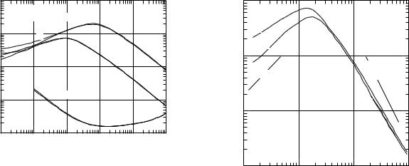
Figure 15.17 shows the mass stopping power for protons, α particles (z = 2, Mα = 4Mp), and electrons and positrons (z = ±1) in carbon as a function of energy. We see a number of features of these curves:

1.All of the stopping power curves have roughly the same shape, rising with increasing energy, reaching a peak, and then falling. (The electron and positron curves peak at a lower energy than is shown in the figure.)

2.There is a region where the stopping power falls approximately as 1/T .

3.At still higher energies the curves rise again. This can be seen for the electron and positron curves above 1 MeV. Similar increases occur in the proton and α- particle curves at higher energies than are plotted here.

The similarities suggest that the stopping power curves for di erent projectiles may be related. Figure 15.18 shows the similarities more clearly. The stopping powers are plotted vs particle speed in the form β = v/c. At low energies (β 1) β is related to kinetic energy by

For larger values of β, the relativistically correct expression

was used to convert Fig. 15.17 to Fig. 15.18. The α- particle stopping power in Fig. 15.17 has been divided

by the square of the α-particle charge number z2 = 4. All three curves of (1/z2)S/ρ vs β are described by very similar functions for β > 0.04, though the electron and α- particle curves are about 10% below the proton curve.4 At low speeds the scaled α-particle curve falls significantly below the proton curve. The reason, the formation of an electron cloud on the α particle, is discussed below.

It is not di cult to understand the basic shape of the stopping power curve. Most of the energy loss is from the projectile to the electrons of the target atom. Since the electrons are bound to the target nucleus, the speed with which the projectile passes the target is important. Imagine pushing slowly on a swing with a force that gradually increases and then decreases. The net force on the swing is the vector sum of the external force exerted Fext, the vertical pull of gravity, and the tension in the ropes and equals the swing’s mass times acceleration. For small horizontal displacements x from equilibrium, the vector sum of the weight and the tension in the string is horizontal and nearly proportional to x. It points toward the equilibrium position, and for small displacements is approximately a linear restoring force. If the proportionality constant is k, ma = Fext − kx.

This is the equation of motion for an undamped harmonic oscillator (Chapter 10 and Appendix F). If the force builds up slowly, there is a very small acceleration, and the swing angle changes so that Fext ≈ kx. As the force decreases the swing returns to its resting position. All of the work that was done to displace the swing is now returned as work by the swing on the source of the external force. No net energy has been imparted to the swing. This is called an adiabatic process or approximation, a slightly di erent use of the term than in Chapter 3.

At the other extreme, the force could be applied for a very short time, building up to a peak and falling quickly. In this case, the swing does not have time to move and Fext = ma. This can be integrated to give

The swing acquires a velocity and hence some kinetic energy. The integral of force with respect to time is called the impulse, and this limit is the impulse approximation.

The two limits depend on whether the duration of the force is long or short compared to the natural period of the swing. The atomic electrons are bound, and they have a natural period that is the circumference of their orbit divided by their speed velectron. The length of time that a projectile exerts a force on the electrons is roughly the diameter of the atom divided by the projectile speed. Ignoring factors of 2π, we see that the passage of the

4A value β = 0.04 corresponds to a kinetic energy of 400 eV for electrons, 800 keV for protons, and 3.2 MeV for α particles.

projectile will be adiabatic if

datom datom vprojectile velectron

or vprojectile velectron. The impulse approximation will

be valid if vprojectile velectron.

This is su cient to explain the shape of the stoppingpower curves in Fig. 15.18. When the projectile has very low energy it moves past the atom so slowly that the electrons have time to rearrange themselves5 and then return to their original state as the projectile leaves, restoring to the projectile the energy that they received while rearranging. As the projectile speed increases, the process is no longer adiabatic, first for the more slowly moving outer electrons and then for more and more of the inner atomic electrons as the speed increases. At the other extreme, when the projectile speed becomes high enough, we can think of the process in terms of the impulse approximation. The faster the projectile moves by, the shorter the time the force is applied and the smaller the energy transfer. The energy transfer is most e ective, and the peak of the stopping power occurs, when the speed of the projectile is about equal to the speed of the atomic electrons in the target.

The cross section dσ/dW in Eqs. 15.45–15.47 is the sum of cross sections for three possible processes. We have already described the stopping power due to interactions of the projectile with the target electrons, Se. There is another contribution to the stopping power from interactions of the projectile with the target nucleus, Sn. It is also possible for the energy loss to involve the radiation of a photon, so we also have radiative stopping power, Sr . Because these are independent processes, the total stopping power and the cross section are each the sum of three terms:

Sρ = Sρe + Sρn + Sρr ,

To compare these processes, we need to consider the maximum energy that can be transferred, as well as the relative probability of each process. The maximum possible energy transfer Wmax can be calculated using conservation of energy and momentum. For a collision of a projectile of mass M1 and kinetic energy T with a target particle of mass M2 which is initially at rest, a nonrelativistic calculation gives

5Classically, if the electrons go around the nucleus many times while the projectile moves by, the shape of their orbits can change in response to the projectile. Quantum-mechanically, the shape of the wave function can change, but the quantum numbers do not change.

The analogous relativistic equation (needed, for example, when the projectile is an electron) is

2(2 + T /M1c2)T M1M2

Wmax = M12 + 2(1 + T /M1c2)M1M2 + M22 . (15.53)

The values of Wmax for representative projectiles and targets are shown in Table 15.3, along with the percentage of the stopping power due to nuclear collisions. For electrons, the table also shows the percentage of the stopping power due to radiative transitions. The percentages are calculated from ICRU Report 49 (1993). Electrons can scatter from nuclei, but the amount of recoil energy transferred to the nucleus is very small. Although electrons undergo a great deal of nuclear scattering, which results in a tortuous path through material, they lose very little energy in a nuclear scattering. The heavier projectiles can lose relatively more energy in each nuclear collision than in each electron collision. For a given kind of projectile, nuclear stopping is more important at lower energies, because less energy can be transferred to an electron. The heavier the projectile for a given energy, the more important the nuclear term becomes, for the same reason.

The collision of electrons with electrons is a special case. Equation 15.52 or 15.53 gives Wmax = T . Consider the collision of two billiard balls of the same mass. If the projectile misses the target, it continues straight ahead with its original energy and W = 0. If it hits the target head on, it comes to rest and the target travels in the same direction with the same energy that the projectile had—a situation indistinguishable from the complete miss. It is customary (but arbitrary) in the case of identical particles to say that the particle with higher energy is the projectile, so Wmax = T /2. This adjustment has been made in Table 15.3 for electrons on electrons and protons on protons.

Radiation is only important for electrons and occurs in a certain fraction of the elastic electron scatterings from the target nucleus. Nuclear scattering gives the electron a fairly large acceleration. Classically, an accelerated charged particle radiates electromagnetic waves. This process is called bremsstrahlung—braking or deceleration radiation. The energy radiated is proportional to the square of the acceleration, so bremsstrahlung is only important for light projectiles. There is also a contribution from electron–electron or positron–electron scattering.

(a)

(b)

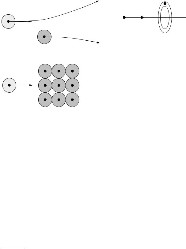
FIGURE 15.19. A projectile, which may or may not carry an electron cloud, moves past a target atom. (a) In a gas the projectile interacts with one atom at a time. (b) In a liquid or a solid, neighboring atoms may influence the interaction.

The electron–electron contribution vanishes at low energies, although the positron–electron bremsstrahlung does not.6 We will see in Chapter 16 that bremsstrahlung is an important component of the x-ray spectrum produced when a beam of electrons strikes a target. Even so, the fraction of the electron energy that is converted to radiation is small.

An atom has a radius of a few times 10−10 m. The nucleus of the atom is much smaller, about 10−15 m, and contains most of the atom’s mass. The atom’s size is determined by the electron cloud around the nucleus. Figure 15.19(a) shows a projectile entering at the left and traveling to the right through a gas. It interacts with one target atom at a time. The solid black dots represent the nuclei of the projectile and the target atom. The shaded circles represent the electron clouds. The projectile may or may not have an electron cloud, which is shown with lighter shading. Figure 15.19(b) shows the interaction with a solid or liquid in which the target atoms

6This di erence can be understood classically. In the first approximation, the radiation by a charge is proportional to the product of the charge times its acceleration, qa. For two interacting electrons, a1 = −a2, q1 = q2, and the sum of these two terms vanishes. For an electron and a positron a1 = −a2, q1 = −q2, and the two terms add.

d σ = 2π b db

FIGURE 15.20. The impact parameter is the perpendicular distance from the target particle to a line extended from the projectile in the direction of its velocity before the interaction.

are tightly packed, and it may not be accurate to say that the projectile interacts with only one atom at a time.

Classically, the motion of a charged projectile past a charged target depends on the charges and masses of the particles, the initial velocity or kinetic energy of the projectile, and the impact parameter b, which is the perpendicular distance from a line through the initial velocity of the projectile to the target, as shown in Fig. 15.20. The classical cross section for having an impact parameter between b and b + db is the area of the ring, 2πb db. If we could relate b to the energy loss W , we would have the cross section dσ/dW of Eq. 15.47.

The energy-loss process is quite complicated, and the cross section cannot be calculated exactly. A great deal of experimental and theoretical work on stopping powers has been done, extending from 1899 to the present time. Di erent models are used for the low energy regime and the high energy regime. The history is nicely reviewed by Ziegler et al. (1985). Much of the recent work on stopping powers has been motivated by the use of ion implantation to make semiconductors, the analysis of materials using ion beams, and medical applications. Currently stopping powers of low-energy heavy ions can be calculated with an accuracy of better than 10%. For high-speed light ions the accuracy is better than 2%. References are found in Ziegler et al. (1985).

15.11.1Interaction with Target Electrons

We first consider the interaction of the projectile with a target electron, which leads to the electronic stopping power, Se. Many authors call it the collision stopping power, Scol. There can be interactions in which a single electron is ejected from a target atom or interactions with the electron cloud as a whole (a “plasmon” excitation). The stopping power at higher energies, where it is nearly proportional to β−2, has been modeled by Bohr, by Bethe, and by Bloch [see the review by Ahlen (1980)]. The Bethe–Bloch model is also valid for relativistic energies. A nonrelativistic model for high energies was developed by J. Lindhard and his colleagues [see references in

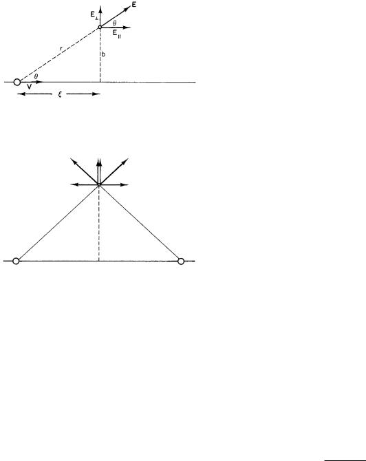
FIGURE 15.21. A heavy particle of charge ze , mass M , and velocity V moves past a stationary electron.

FIGURE 15.22. Why the parallel component of p is zero. For every point where the projectile gives a particular E , there is a symmetric point where E is equal but opposite. The components E are in the same direction in both places, so the perpendicular component of p does not vanish.

tile that gives a parallel component of F in one direction, there is a position an equal distance on the other side of the point of closest approach that gives a component of F with the same magnitude but in the opposite direction. The perpendicular component of F is the same for both locations, so there is a net perpendicular component of momentum transfer. The magnitude of the perpendicular component of E is

change during the collision. The magnitude of the impulse is therefore

The smaller the impact parameter, the greater the momentum transfer to the electron. The kinetic energy acquired by the electron is

Ziegler et al. (1985)]. It allows more accurate calculations of which electrons in the target receive energy from the projectile.

We can gain considerable insight into the high-energy loss process by making a classical calculation of the cross section for transferring energy to an electron using the impulse approximation. This is a simplification of the Bethe–Bloch model. In our model, a heavy projectile passes by a free electron that is at rest. Momentum is transferred from the projectile to the electron. Because of its large mass, the projectile’s velocity does not change appreciably, but the lighter electron acquires an appreciable velocity and kinetic energy. If the momentum transferred to the electron is p, its kinetic energy is p2/2me. That kinetic energy must have been lost by the projectile.

Figure 15.21 shows a particle of mass M , charge ze, and velocity V = βc moving past a stationary electron. The impact parameter b is the perpendicular distance from the electron to the path of the projectile. The distance from the projectile to the electron is r, and the distance along the path to the point of closest approach is ξ. The momentum transferred to the electron is

p = Fdt = −e Edt. By symmetry, there is no component of p parallel to the path of the projectile. The reason is shown in Fig. 15.22. For each location of the projec-

The factor e4/(4π 0)2mec2 depends only on the charge and mass of the electron. It can be written as re2mec2, where re is the classical radius of the electron [Eq. 15.18]. The factor has the numerical value

re2mec2 = 6.50 × 10−43 J m2 = 4.06 × 1024 eV m2.

Using this notation the energy transfer per target electron is

2z2r2mec2

W = e . (15.54)

β2b2

Here z is the charge on the projectile, βc is its speed, and b is the impact parameter. Note that W does not depend on the mass of the heavy projectile, but only on its speed. As the speed becomes less, the energy transfer becomes greater, because the projectile takes longer to move past the electron and the force is exerted for a longer time (as long as the time is still short enough so that the impulse approximation remains valid).

If the electrons are uniformly distributed, the cross section for each electron is dσ = (dσ/dW )dW = 2πb db. This can be written, with the help of Eq. 15.54, in terms of W :

This expression diverges as W approaches zero, corresponding to very large impact parameters. However, the assumption that the target electrons are free fails in this limit, so that there is some e ective lower limit Wmin. Also, the greater the impact parameter, the longer the electron will experience the force exerted by the projectile (though it will be weaker). If the time is too long, the electron can move in response to the force and not absorb as much energy; the impulse approximation is no longer valid. We have already seen that there is a maximum energy transfer Wmax. Multiplying the cross section by W , integrating from Wmin to Wmax, and noting that there are Z electrons per target atom, we obtain

The factor 4πNAre2mec2 has the value 30.707 eV m2 mol−1 = 0.307 07 MeV cm2 mol−1.

A quantum-mechanical calculation gives a result of essentially the same form as Eq. 15.56. The logarithmic term includes both ionization and plasmon excitation7 and is called the stopping number per atomic electron

Equation 15.57 with L = L0 is often called the Bethe– Bloch formula. The second term in L0 depends on I(Z), the ionization potential of the atoms in the absorber, averaged over all the electrons in the atom. Values of I(Z) have been calculated theoretically and also derived from measurements of the stopping power. They range from 14.8 eV for hydrogen to 884 eV for uranium. The value 14.8 eV is greater than the ground-state energy of hydrogen, 13.6 eV, because the ejected electron has some average kinetic energy.

Published values of I can vary considerably, depending on whether the other correction terms are present. For example, values of I in the literature for hydrogen range from 11 to 20 eV. Discussions of values for I and the various terms in L can be found in ICRU Report 49 (1993), in Ahlen (1980), and in Attix (1986). The term δ/2 corrects for the density e ect. The calculation above assumed that the electron experienced the full electric field of the projectile. However, other electrons in the absorber move slightly, polarizing the absorber and reducing the field. This e ect becomes important at high

7A plasmon excitation is due to the interaction of the projectile with the entire electron cloud of the atom.

energies as the electric field is distorted by relativistic effects. It also depends on the density of the absorber. A small density e ect persists in conductors even at low energies; however, it is usually incorporated into the value of I(Z). For the projectile energies we are considering, the density e ect is most important for electrons.

An alternative nonrelativistic treatment by Lindhard and colleagues allows the use of accurate atomic electron density distributions and also considers the e ect of electrons in neighboring atoms.8 In the Lindhard model the stopping power is

where z is the projectile charge, I is the stopping interaction strength in J m2 (more often in eV pm2),9 ρe is the electron density in the atom (in units of the electron charge), and 4πr2dr is the volume element. Integration of ρe over all volume gives Z, the atomic number of the target. Comparison of Eqs. 15.59 and 15.47 shows that the integral in Eq. 15.59 is the stopping cross section per target atom.

Figure 15.23 shows how the Lindhard model explains why the stopping power falls below the 1/β2 curve at lower projectile velocities. Each panel shows the electron density in copper, 4πr2ρe, and the interaction strength I. Their product, the solid line, is the integrand in Eq.

˚

15.59. The integral is taken from 0 to 0.14 nm (1.4 A (angstrom)). The K, L, and M shells of copper can be seen in the electron density curve. Figure 15.23(a) is for a 10-MeV proton or some other heavy ion with the same speed. The projectile is moving fast enough so that all electrons except those in the K shell interact with it. Contrast this with Fig. 15.23(b), which is for a 100-keV proton. The projectile speed is much less, and the interaction is almost exclusively with the outer electrons.10

Both the Bethe–Bloch and Lindhard models fail at low energy, because the electrons are not free and many of the interactions are adiabatic. Some models reviewed by Ziegler et al. (1985) predict a stopping power proportional to projectile velocity. This has been found to be true in general, though not for all elements. The experiments are quite di cult because of the thinness of the targets, contamination, and so on. Figure 15.24 shows the regions where the various models apply for protons. For electrons, relativistic e ects are important above about

8The electron density functions are calculated using quantum mechanics. The problem is to find the electron distribution by solving Schr¨odingers equation with the potential distribution due to the nucleus and the potential due to the electron charge distribution for which one is solving. This self-consistent computation is called the Hartree–Fock approximation.

9I is not the same as the average ionization energy of Eq. 15.58. 10The solid line representing the integrand does not fall to zero at

˚

0.12 nm = 1.2 A because of the e ect of electrons from neighboring atoms. In a solid there are no regions where the electron density is zero.