

Intermediate Physics for Medicine and Biology - Russell K. Hobbie & Bradley J. Roth
.pdf(a) |
(b) |
FIGURE 18.11. The z components of the magnetic moments of two protons in a water molecule are shown for two di erent molecular orientations, (a) and (b). When the water molecule is fixed in space, as in ice, the magnetic field that one proton produces in the neighborhood of the other is static. When the water molecule tumbles, as in a liquid or gas, the field that one proton produces at the other changes with time.
TABLE 18.2. Approximate relaxation times at 20 MHz.
|
T1 (ms) |
T2 (ms) |
Whole blood |
900 |
200 |
Muscle |
500 |
35 |
Fat |
200 |
60 |
Water |
3,000 |
3,000 |
|
|
|
of each magnetic field component is exponential and that each field component has the same correlation time τC :
φ11(τ ) e−|τ |/τC . |
(18.33) |
The Fourier transform of the autocorrelation function gives the power at di erent frequencies. It has only cosine terms because the autocorrelation is even. Comparison with the Fourier transform pair of Eq. 11.100 shows that the power at frequency ω is proportional to τC /(1+ω2τC2 ). With the assumption that the transition rate, which is 1/T1, is proportional to the power at the Larmor frequency, we have [see also Slichter (1978), p. 167, or Dixon et al. (1985)]
|
1 |
= |
CτC |
|
, |
(18.34) |
|
1 + ω02 |
τC2 |
||||
T1 |
|
|
||||
where C is the proportionality constant.
The correlation time in a solid is much longer than in a liquid. For example, in liquid water at 20 ◦C it is about 3.5 × 10⁻¹² s; in ice it is about 2 × 10⁻⁶ s. Figure 18.12 shows the behavior of T1 as a function of correlation time, plotted from Eq. 18.34 with C = 5.43×10¹⁰ s−2. For short correlation times T1 does not depend on the Larmor frequency. At long correlation times T1 is proportional to the Larmor frequency, as can be seen from Eq. 18.34. The minimum in T1 occurs when ω0 = 1/τC in this model.
Table 18.2 shows some typical values of the relaxation times for a Larmor frequency of 20 MHz. Neighboring
18.6 Relaxation Times |
523 |
|
102 |
|
|
|
|
|
|
|
|
101 |
Water at 20¡ C |
|
T1 at 29 MHz |
|
|||
|
|
|
|
|
|
|
||
|
100 |
|
|
|
|
|
|
|
, s |
10-1 |
|
|
|
|
|
|
|
|
|
|
|
|
|
|
|
|
2 |
|
|
|
|
|
|
|
|
T |
10-2 |
|
|
|
T1 at 10 MHz |
|
||
or |
|
|
|
|
||||
1 |
|
|
|
|
|
|
|
|
T |
10-3 |
|
|
|
|
|
|
|
|
|
|
|
|
|
|
||
|
10 |
-4 |
|
|
|
|
Ice |
|
|
|
|
|
|
|
|
|
|
|
|
|
|
|
|
|
T2 |
|
|
10-5 |
|
|
|
|
|
|
|
|
10-6 |
10-11 10-10 |
10-9 |
10-8 |
10-7 |
10-6 |
10-5 |
|
|
|
10-12 |
||||||
Correlation time, s
FIGURE 18.12. Plot of T1 and T2 vs correlation time of the fluctuating magnetic field at the nucleus. The dashed lines are for a Larmor frequency of 29 MHz; the solid lines are for 10 MHz. Experimental points are shown for water (open dot) and ice (solid dots).
paramagnetic atoms reduce the relaxation time by causing a fluctuating magnetic field. For example, adding 20 ppm of Fe3+ to pure water reduces T1 from 3,000 to 20 ms.
Di erences in relaxation time are easily detected in an image. Di erent tissues have di erent relaxation times. A contrast agent containing gadolinium (Gd3+), which is strongly paramagnetic, is often used in magnetic resonance imaging. It is combined with many of the same pharmaceuticals used with 99mTc, and it reduces the relaxation time of nearby nuclei.
The hemoglobin that carries oxygen in the blood exists in two forms: oxyhemoglobin and deoxyhemoglobin. The former is diamagnetic and the latter is paramagnetic, so the relaxation time in blood depends on the amount of oxygen in the hemoglobin. The imaging technique that exploits this is called BOLD (blood oxygen level dependent).
The same model for the fluctuating fields which led to Eq. 18.34 gives an expression for T2:
1 |
= |
|
CτC |
+ |
1 |
, |
|
(18.35) |
||
T2 |
|
|
2 |
|
|
|
2T1 |
|
||
|
|
|
2 |
|
|
1 + ω02τC2 |
|
|||
T2 = |
|
|
|
|
. |
|
||||
CτC |
|
|
2 + ω02τC2 |
|
||||||
There is a slight frequency dependency to T2 for values of the correlation time close to the reciprocal of the Larmor frequency.
Another e ect that causes the magnetization to rapidly decrease is dephasing. Dephasing across the sample occurs because of inhomogeneities in the externally-applied field. Suppose that the spread in Larmor frequency and
524 18. Magnetic Resonance Imaging
the transverse relaxation time are related by T2∆ω = K. (UsuallyK is taken to be 2.) The spread in Larmor frequencies ∆ω is due to a spread in magnetic field ∆B experienced by the nuclear spins in di erent atoms. The total variation in B is due to fluctuations caused by the magnetic field of neighbors and to variation in the applied magnetic field across the sample:
∆Btot = ∆Binternal + ∆Bexternal.
Therefore
∆ωtot = ∆ωinternal + ∆ωexternal.
The total spread is associated with the experimental relaxation time, T2 = K/∆ωtot. The “true” or “nonrecoverable” relaxation time T2 = K/∆ωinternal is due to the fluctuations in the magnetic field intrinsic to the sample. Therefore
1 |
= |
1 |
+ |
γ∆Bexternal |
. |
(18.36) |
T |
T2 |
|
||||
|
|
K |
|
|||
2 |
|
|
|
|
|
|
T2 is called the nonrecoverable relaxation time because various experimental techniques can be used to compensate for the external inhomogeneities, but not the internal atomic ones.
18.7Detecting the Magnetic Resonance Signal
We have now seen that a sample of nuclear spins in a strong magnetic field has an induced magnetic moment; that it is possible to apply a sinusoidally varying magnetic field and nutate the magnetic moment to precess at any arbitrary angle with respect to the static field; and that the magnetization then relaxes or returns to its original state with two characteristic time constants, the longitudinal and transverse relaxation times. We next consider how a useful signal can be obtained from these spins. This is done by measuring the weak magnetic field generated by the magnetization as it precesses in the xy plane.
Suppose that a sample is at the origin. The motions plotted in Fig. 18.7 suggest that one way to produce a magnetization rotating in the xy plane is to have a static field along the z axis, combined with a coil in the yz plane (perpendicular to the x axis) connected to a generator of alternating current at frequency ω0. Turning on the generator for a time ∆t = π/2ω1 = π/γB1 rotates the magnetization into the xy plane (a 90 ◦ or π/2 pulse). If the generator is then turned o , the same coil can be used to detect the changing magnetic flux due to the rotating magnetic moments. The resulting signal, an exponentially damped sine wave, is called the free induction decay (FID).
To estimate the size of the signal induced in the coil, imagine a magnetic moment µ = M∆V rotating in the xy plane as shown in Fig. 18.13. The voltage v induced
z
y
x
Coil
FIGURE 18.13. A magnetic moment rotating in the xy plane induces a voltage in a pickup coil in the yz plane. The coil is viewed from slightly to the right of the coil.
z
y  Br
Br
θ
x |
x |
Coil
FIGURE 18.14. A dipole along the x axis generates a flux through the shaded circle in the yz plane that is equal and opposite to that through the hemispherical cap. The drawing is viewed from slightly to the right of the yz plane.
in a one-turn coil in the yz plane is the rate of change of the magnetic flux through the coil:
v = −∂∂tΦ = −∂t∂ B · dS.
The magnetic field far from a magnetic dipole can be written most simply in spherical coordinates [Eqs. 18.32]. We need the flux through the coil of radius a in the yz plane. However, Eqs. 18.32 are not valid close to the dipole. Since a fundamental property of the magnetic field
is that for a closed surface B ·dS = 0, the flux through the coil in Fig. 18.13 is the negative of the flux Φ through
the hemispherical cap in Fig. 18.14:
Φ = − |
|
|
|
2 |
|
µ0 4πµx |
π/2 |
|
||
|
Br 2πa |
sin θ dθ = − |
|
|
|
|
cos θ sin θ dθ |
|||
|
4π |
a |
0 |
|||||||
= − |
µ0 2πµx |
. |
|
|
|
|
|
(18.37) |
||
4π |
|
a |
|
|
|
|
|
|||
At any instant µ can be resolved into components along x and y. The component pointing along y contributes no net flux through the spherical cap of Fig. 18.14. Therefore, the flux for a magnetic moment µ = M∆V , where M is given by Eqs. 18.16, is
Φ = −µ0 2πM0∆V e−t/T2 cos(−ω0t).
4π a
|
|
|
|
18.8 Some Useful Pulse Sequences |
525 |
||||||
Pulse |
|
π/2 |
|
|
|
|
|
|
|
|
|
|
|
|
|
|
|
|
|
|
|||
|
|
|
|
|
π/2 |
|
|
|
|||
|
|
|
|
|
|
|
|
|
|
|
|
|
|
|
|
|
|
|
|
|
|
|
|
|
|
|
|
|
|
|
|
|
|
|
|
|
|
|
|
|
TR |
|
|
|
|
|
|
|
|
|
|
|
|
|
|
||||
Mz |
1-e-t/T1 |
The induced voltage is −∂Φ/∂t:
v = |
µ0 2πM0∆V |
1 |
|
|||
|
|
|
e−t/T2 − |
|
cos(−ω0t) + ω0 sin(−ω0t) . |
|
4π |
a |
T2 |
||||
Since 1/T2 ω0, this can be simplified to
Mx |
e |
-t/T2* |
|
|
v = |
− |
µ0 ω0 |
2πM |
∆V e−t/T2 sin( |
− |
ω |
t). |
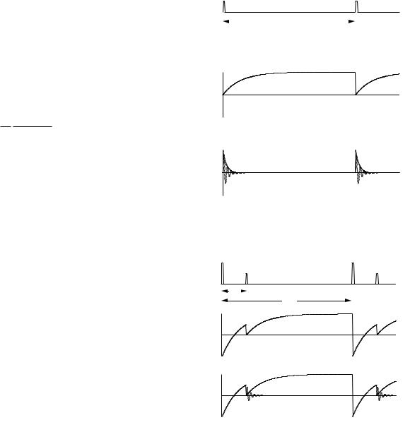
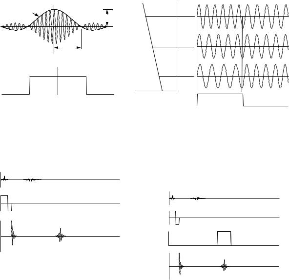
FIGURE 18.15. Pulse sequence and signal for a free-induc- |
|||
|
|
|
|||||||||
4π a |
|||||||||||
|
0 |
|
0 |
|
tion-decay measurement. |
||||||
If the value of Mz which exists at thermal equilibrium has been nutated into the xy plane, then M0 is given by
the Mz of Eq. 18.10. For a spin- 1 |
particle (and using the |
|||||
|
|
|
|
2 |
|
|
fact that ω0 = γB0) we obtain |
|
|||||
|
µ0 πN ∆V γ3 2B2 |
|
||||
v = − |
|
|
|
0 |
e−t/T2 sin(−ω0t). (18.38) |
|
4π |
2kB T a |
|
||||
Here N ∆V is the total number of nuclear spins involved, B0 is the field along the z axis, and a is the radius of the coil that detects the free-induction-decay signal. For a volume element of fixed size, as in magnetic resonance imaging, the sensitivity is inversely proportional to the coil radius. If the sample fills the coil, as in most laboratory spectrometers, then ∆V a2 and the sensitivity is proportional to a.
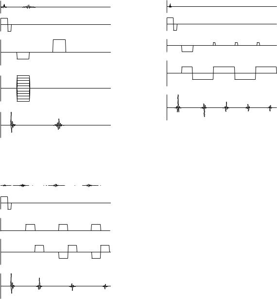
18.8 Some Useful Pulse Sequences
Many di erent ways of applying radio-frequency pulses to generate B1 have been developed by nuclear magnetic resonance spectroscopists for measuring relaxation times. There are five “classic” sequences, which also form the basis for magnetic resonance imaging.
18.8.1 Free-Induction-Decay (FID) Sequence
Free induction decay was described in Sec. 18.7. A π/2 pulse nutates M into the xy plane, where its precession induces a signal in a pickup coil. The signal is of the form e−(t/T2 ) sin(−ω0t), where T2 is the experimental transverse relaxation time, including magnetic field inhomogeneities due to the apparatus as well as those intrinsic
Pulse |
π |
π |
|
π/2 |
π/2 |
||
|
|||
|
TI |
TR |
|
|
|
||
Mz |
|
|
|
Mx |
|
|
FIGURE 18.16. The inversion recovery sequence allows determination of T1 by making successive measurements at various values of the interrogation time TI .
to the sample. Figure 18.15 shows the pulse sequence, the value of Mx, and the value of Mz . The signal is proportional to Mx. The pulses can be repeated after time TR for signal averaging. It is necessary for TR to be greater than, say, 5T1 in order for Mz to return nearly to its equilibrium value between pulses.
18.8.2Inversion-Recovery (IR) Sequence
The inversion-recovery sequence allows measurement of T1. A π pulse causes M to point along the −z axis. There
526 18. Magnetic Resonance Imaging
|
y' |
|
|
y' |
Pulse π/2 |
π |
π/2 |
π |
|
|
|
|
|
||||
a |
|
|
|
θ |
|
|
|
|
b |
x' |
a |
b |
x' |
|
TR |
|
|
Mz |
(a) |
(b) |
y' |
y' |
|
Mx |
e |
(-t/T2) |
|
|
|
|
x' |
x' |
|
|
a |
b |
a b |
(c) |
(d) |
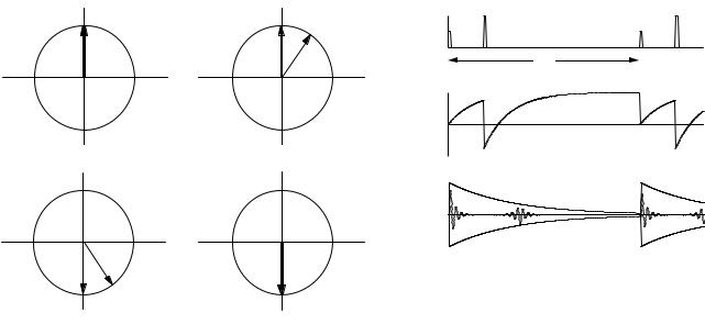
FIGURE 18.17. Two magnetic moments are shown in the x y plane in the rotating coordinate system. Moment a rotates at the Larmor frequency and remains aligned along the y axis. Moment b rotates clockwise with respect to moment a. (a) Both moments are initially in phase. (b) After time TE /2 moment b is clockwise from moment a. (c) A π pulse nutates both moments about the x axis. (d) At time TE both moments are in phase again.
is not yet any signal at this point. Mz returns to equilibrium according to Mz = M0 1 − 2e−(t/T1) . A π/2 interrogation pulse at time TI rotates the instantaneous value of Mz into the xy plane, thereby giving a signal proportional to M0 1 − 2e−(TI /T1) , as shown in Fig. 18.16. The process can be repeated; again the repeat time must exceed 5T1.
You can see from Fig. 18.16 that there will be no signal at all if TI /T1 = 0.693. If TI is less than this, the Mx signal will be inverted (negative). Unless special detector circuits are used which allow one to determine that Mx is negative, the results can be confusing.
Inversion recovery images take a long time to acquire and there is ambiguity in the sign of the signal. There are also problems with the use of a π pulse for slice selection [defined in Sec. 18.9; the details of the problems are found in Joseph and Axel (1984)].
18.8.3 Spin–Echo (SE) Sequence
The pulse sequence shown in Fig. 18.17 can be used to determine T2 rather than T2 . Initially a π/2 pulse nutates M about the x axis so that all spins lie along the rotating y axis. Figure 18.17(a) shows two such spins. Spin a continues to precess at the same frequency as the rotating coordinate system; spin b is subject to a slightly smaller magnetic field and precesses at a slightly lower frequency, so that at time TE /2 it has moved clockwise in the rotat-
FIGURE 18.18. The pulse sequence and magnetization components for a spin–echo sequence.
ing frame by angle θ, as shown in Fig. 18.17(b). At this time a π pulse is applied that rotates all spins around the x axis. Spin a then points along the −y axis; spin b rotates to the angle shown in Fig. 18.17(c). If spin b still experiences the smaller magnetic field, it continues to precess clockwise in the rotating frame. At time TE both spins are in phase again, pointing along −y as shown in Fig. 18.17(d). The resulting signal is called an echo, and the process for producing it is called a spin-echo sequence. The formation of an echo depends only on the fact that the magnetic field at the nucleus remained the same before and after the π pulse; it does not depend on the specific value of the dephasing angle. Therefore, all of the spin dephasing that has been caused by a timeindependent magnetic field is reversed in this process. There remains only the dephasing caused by fluctuating magnetic fields. Figure 18.18 shows the pulse sequence and signal.
18.8.4Carr–Purcell (CP) Sequence
When a sequence of π pulses that nutate M about the x axis are applied at TE /2, 3TE /2, 5TE /2, etc., a sequence of echoes are formed, the amplitudes of which decay with relaxation time T2. This is shown in Fig. 18.19. Referring to Fig. 18.17, one can see that the echoes are aligned alternately along the −y and +y axes. One advantage of the Carr–Purcell sequence is that it allows one to determine rapidly many points on the decay curve. Another advantage relates to di usion. The molecules that contain the excited nuclei may di use. If the external magnetic field B0 is not uniform, the molecules can di use to another region where the magnetic field is slightly di erent. As a result the rephasing after a pulse does not completely cancel the initial dephasing. This e ect is reduced by the Carr–Purcell sequence (see Problem 38).
Pulse |
|
|
|
|
|
|
|
|
|
|
|
|
π |
||||
|
π/2 |
π |
|
|
|||||||||||||
|
|
π |
π |
|
|
||||||||||||
|
|
|
|
|
|
|
|
|
|
|
|
|
|
|
|
|
|
|
|
|
|
|
|
|
|
|
|
|
|
|
|
|
|
|
|
|
|
TE/2 |
|
|
TE |
|
|
|
TE |
|
|
TE |
|||||
Mz |
Mx |
e(-t/T2) |
|
|
|
|
|
|
|
|
|
|
|
|
18.9 Imaging |
527 |
|||||
|
|
|
|
|
|
|
|
|
|
|
|
|
|
|
|
|||
Pulse |
|
|
|
|
|
|
|
π(y') |
|
π(y') |
||||||||
|
π/2 |
π(y') |
π(y') |
|
|
|||||||||||||
|
|
|
|
|
|
|
|
|
|
|
|
|
|
|
|
|
|
|
|
|
|
|
|
|
|
|
|
|
|
|
|
|
|
|
|
|
|
|
|
TE/2 |
TE |
|
|
TE |
|
|
TE |
|
|
|
||||||
Mz |
Mx |
e(-t/T2) |
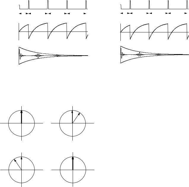
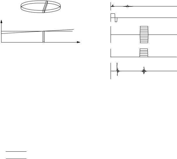
FIGURE 18.19. The Carr–Purcell pulse sequence. All pulses nutate about the x axis. Echoes alternate sign. The envelope of echoes decays as e−t/T2 , where T2 is the unrecoverable transverse relaxation time.
|
y' |
|
|
y' |
|
a |
b |
x' |
a |
b |
x' |
|
|
|
|
(a) |
(b) |
y' |
y' |
FIGURE 18.21. The CPMG pulse sequence.
quence overcomes this problem. The initial π/2 pulse nutates M about the x axis as before, but the subsequent pulses are shifted a quarter cycle in time, which causes them to rotate about the y axis. This is shown in Fig. 18.20. To see why this pulse sequence is less sensitive to errors in the duration of the π pulses, consider moment a. In the CP sequence, Fig. 18.17, a π pulse that is too long will nutate a too far, and it will have a smaller component in the x y plane. The next pulse will nutate it even further. In Fig. 18.20, the π pulses will not a ect moment a at all. This is explored further in Problems 26 and 27.
b |
a |
x' |
a b |
x' |
(c) |
(d) |
FIGURE 18.20. The e ect of the Carr–Purcell–Meiboom–Gill pulse sequence on the magnetization. This is similar to Fig. 18.17 except that the π pulses rotate around the y axis. Moment b rotates clockwise in the x y plane. (a) Both moments are initially in phase. (b) After time TE /2 moment b is clockwise from moment a. (c) A π pulse rotates both moments about the y axis. (d) At time TE both moments are in phase again.
18.8.5Carr–Purcell–Meiboom–Gill (CPMG) Sequence
One disadvantage of the CP sequence is that the π pulse must be very accurate or a cumulative error builds up in successive pulses. The Carr–Purcell–Meiboom–Gill se-
18.9 Imaging
Many more techniques are available for imaging with magnetic resonance than for x-ray computed tomography. They are described by Joseph (1985), by Cho et al. (1993), by Vlaardingerbroek and den Boer (2002), and by Liang and Lauterbur (2000). One of these authors, Paul C. Lauterbur, shared with Sir Peter Mansfield the 2003 Nobel Prize in Physiology or Medicine for the discovery of magnetic resonance imaging.
Creation of the images requires the application of gradients in the static magnetic field Bz which cause the Larmor frequency to vary with position. The first gradient is applied in the z direction during the π/2 pulse so that only the spins in a slice in the patient are selected (nutated into the xy plane). Slice selection is followed by gradients of Bz in the x and y directions. These also change the Larmor frequency. If the gradient is applied during the readout, the Larmor frequency of the signal varies as Bz varies with position. If the gradient is applied before the readout, it causes a position-dependent phase shift in the signal which can be detected.
528 18. Magnetic Resonance Imaging
During π / 2
pulse |
z |
z |
B z
(a) |
(b) |
(c) |
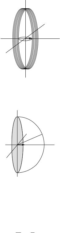
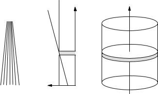
FIGURE 18.22. (a) Magnetic field lines for a magnetic field that increases in the z direction. (b) A plot of Bz vs z with and without a gradient. (c) After application of a field gradient in the z direction during the specially shaped rf pulse, all of the spins in the shaded slice are excited, that is, they are precessing in the xy plane.
We discuss several reconstruction methods here. Projection reconstruction is similar to CT reconstruction, but is slow and rarely used. A two-dimensional Fourier technique known as spin warp or phase encoding forms the basis of the techniques used in most machines. We also describe briefly some techniques that are even faster. Finally, we discuss how the image contrast can be modified by changing the pulse sequence parameters.
Our initial discussion is based on a spin–echo pulse sequence, repeated with a repetition time TR as shown in Fig. 18.18.
18.9.1 Slice Selection
First, suppose we simply apply a π/2 pulse to the entire sample in a 1.5-T machine (ω0 = 401 ×106 s−1; ν0 = 63.9 MHz). If the duration of this pulse is to be, say, 5 ms, it requires a constant amplitude of the radio-frequency magnetic field
B1 = π/γ∆t = 2.35 × 10⁻⁶ T. |
(18.39) |
The pulse lasts for 3×10⁵ cycles at the Larmor frequency. The frequency spread of the pulse is about 200 Hz. This excites all the proton spins in the entire sample.
For MR imaging, we want to select a thin slice in the sample. In order to select a thin slice (say ∆z = 1 cm) we apply a magnetic field gradient in the z direction while applying a specially shaped B1 signal. In a static magnetic field B0, the field lines are parallel. The field strength is proportional to the number of lines per unit area and does not change. With the gradient applied in the volume of interest, the field lines converge, and the field increases linearly with z as shown in Figs. 18.22(a)
and 18.22(b):
Bz (z) = B0 + Gz z. |
(18.40) |
We adopt a notation in which G represents a partial derivative of the z component of the magnetic field:
Gx |
|
∂Bz /∂x |
|
|
G = Gy |
= ∂Bz /∂y |
. |
(18.41) |
|
|
|
|
|
|
Gz |
|
∂Bz /∂z |
|
|
In a typical machine, Gz = 5 × 10⁻³ T m−1. For a slice thickness ∆z = 0.01 m, the Larmor frequency
across the slice varies from ω0 − ∆ω to ω0 + ∆ω, where ∆ω = γGz ∆z/2 = 6.68 × 10³ s−1 (∆f = 1.064 kHz).
It is possible to make the signal Bx(t) consist of a uniform distribution of frequencies between ω0 − ∆ω and ω0 + ∆ω, so that all protons are excited in a slice of thickness ∆z from −∆z/2 to +∆z/2. Let the amplitude of Bx in the interval (ω, dω) be A. Using Eq. 11.55, Bx(t) is given by
Bx(t) = |
A |
ω0+∆ω cos(ωt) dω |
|
|||||
|
|
|||||||
|
2π |
ω0 |
−∆ω |
|
||||
|
|
|
|
|||||
= |
A∆ω |
|
sin(∆ωt) |
cos(ω0t). |
(18.42) |
|||
|
|
|||||||
|
π |
|
|
|
∆ωt |
|
||
This has the form B1(t) cos(ω0t), where B1(t) = (A∆ω/π) sin(∆ωt)/(∆ωt). The function sin(x)/x has its maximum value of 1 at x = 0. It is also called the sinc(x) function. The angle φ through which the spins are nutated is
φ = |
∞ ω1(t) dt = |
|
γ |
∞ B1(t) dt |
||||||
2 |
||||||||||
|
|
−∞ |
|
|
−∞ |
|||||
|
|
∞ |
|
|
|
|||||
= |
|
γA∆ω |
sin(∆ωt) |
dt |
||||||
2π |
|
|||||||||
|
|
−∞ |
∆ωt |
|||||||
|
|
γA |
|
|
|
|
|
|||
= |
|
. |
|
|
|
|
|
|
||
2 |
|
|
|
|
|
|
||||
|
|
|
|
|
|
|
|
|||
For a π/2 pulse, A = π/γ. The maximum value of B1 is therefore ∆ω/γ = Gz ∆z/2, as shown in Fig. 18.23. The Bx pulse does not have an abrupt beginning; it grows and decays as shown. In practice, it is truncated at some distance from the peak where the lobes are small.
While the gradient is applied, the transverse components of spins at di erent values of z precess at di erent rates (see Problem 32). Therefore it is necessary to apply a gradient Gz of opposite sign after the π/2 pulse is finished in order to bring the spins back to the phase they had at the peak of the slice selection signal. The gradient is removed when all of the spins in the slice shown in Fig. 18.22(c) are back in phase. They then continue to precess in the xy plane at the Larmor frequency. This gives the first Mx pulse in Fig. 18.24. This initial free-induction- decay pulse is not used for imaging.
The voltage induced in the pickup coil surrounding the sample is proportional to the free induction decay of M in the entire slice. That is, the voltage signal induced in
|
Bx(t ) |
|
|
B1(t) |
A ∆ω/π |
|
|
= ∆ω/γ = Gz |
∆z/2 |
||
|
|||
|
t |
|
|
|
π/∆ω |
B0, ω0 |
|
|
= 2π/γ Gz ∆z |
|
|
|
C(ω) |
|
18.9 Imaging |
529 |
x or y
ω0 − ∆ω |
ω0 |
ω0 |
+ ∆ω |
Bz |
Gradient |
|
|
= ω0 |
+ γGz∆z/2 |
|
|
FIGURE 18.23. (a) The Bx(t) signal shown is used to selectively excite a slice. It consists of cos(ω0t) modulated by a sinc(x) or sin(x)/x pulse B1(t). (b) The frequency spectrum contains a uniform distribution of frequencies.
π/2 π Bx 


Gz
Mx |
FIGURE 18.24. A slice selection pulse sequence. While a gradient Gz is applied, a π/2 Bx (rf) pulse nutates the spins in a slice of thickness z into the xy plane. A negative Gz gradient restores the phase of the precessing spins. The echo after the π pulse is from the entire slice.
the pickup coil is proportional to M (x, y, z) cos(−ω0t) f (t) dV , where M (x, y, z) is the magnetization per unit volume that was nutated into the xy plane, cos(−ω0t) represents the change in signal as M rotates in the xy plane at the Larmor frequency, and f (t) represents relaxation, signal buildup during an echo, and so on. Figure 18.24 shows the echo after a subsequent π pulse.
We assume that changes in f (t) are slow compared to the Larmor frequency and neglect them here. Then the
signal from an element dxdy in the slice is |
|
v(t) = A dx dy ∆z M (x, y, z) cos(−ω0t). |
(18.43) |
Constant A includes all the details of the detecting coils and receiver.
FIGURE 18.25. A gradient in Bz causes the Larmor frequency to vary with position. If the signal is measured while the gradient is applied, the Larmor frequency varies with position. If the signal is measured after the gradient has been applied and removed, a position-dependent phase shift remains.
π/2 π Bx 


Gz
Gx
Mx |
FIGURE 18.26. A gradient Gx is applied during x readout. The echo signal between ω and ω + dω is proportional to the magnetization in a strip between x and x+dx, integrated over all values of y.
18.9.2 Readout in the x Direction
We now need to extract x and y position information from v(t). This is done by creating gradients of Bz in the x or y directions. As shown in Fig. 18.25, if the signal is measured while a gradient is applied, the Larmor frequency varies with position. Suppose that Bz is given a gradient Gx in the x direction during the echo signal readout, as shown in Fig. 18.26. The spins that echo in the shaded slice between x and x + dx in Fig. 18.27 will be precessing with a Larmor frequency between ω and ω + dω, where
530 18. Magnetic Resonance Imaging
B z
x
FIGURE 18.27. Because the gradient Gx is applied during readout, the Larmor frequency of all spins in the shaded slice is between ω and ω + dω.
ω = ω0 + γGxx. The signal from the entire slice is
|
|
v(t) = A∆z dx dy M (x, y, z) cos[−ω(x)t].
(18.44) We use the fact that ω(x) = ω0 +γGxx to write the signal as
|
|
|
v(t) = A∆z dx dy M (x, y, z) cos(−ω0t − γGxxt) .
(18.45)
Since the z slice has already been selected, let us simplify the notation by dropping the z dependence of M. The electronics in the detector multiply v(t) by cos(ω0t) or sin(ω0t) and average over many cycles at the Larmor frequency. The results are two signals that form the basis for constructing the image:
sc(t) = v(t) cos(ω0t) dx dy M (x, y) cos(−γGxxt),
ss(t) = v(t) sin(ω0t) dx dy M (x, y) sin(−γGxxt).
(18.46)
The time average is over many cycles at the Larmor frequency but a time short compared to 2π/γGxxmax.
18.9.3 Projection Reconstruction
By inspecting Eq. 18.46 and remembering the relationship between ω and x, we see that the Fourier transforms
of sc(t) and ss(t) are both proportional to M (x, y) dy. (Of course, the signals are digitized and one actually deals with discrete transforms.) This means that sc or ss can be Fourier analyzed to determine the amount of signal in the frequency interval (ω, dω) corresponding to (x, dx), which
is proportional to the projection M (x, y) dy along the shaded strip. In Sec. 12.5 we learned how to reconstruct an image from a set of projections. The entire readout process can therefore be repeated with the gradient rotated slightly in the xy plane (that is, with a combination of Gx and Gy during readout). This is indicated in Fig. 18.28, which indicates many scans, with di erent values of Gx and Gy , related by Gx/Gy = tan θ, where θ is
π/2 π Bx 


Gz
Gx
Gy
Mx |
FIGURE 18.28. Projection reconstruction techniques can be used to form an image. A series of measurements are taken, each with simultaneous gradients Gx and Gy .
the angle between the projection and the x axis. All of the techniques for reconstruction from projections that were developed for computed tomography can be used to reconstruct M (x, y). Sending the proper combination of currents through the x and y gradient coils rotates the gradient; no rotating mechanical components are needed.
18.9.4Phase Encoding
Techniques are available for magnetic resonance imaging that are not available for computed tomography. They are based on determining directly the Fourier coe cients in two or three dimensions. The basic technique is called spin warp or phase encoding. We saw in Fig. 18.25 that if a gradient is applied after the π/2 slice-selection pulse, a position-dependent phase shift remains even after the gradient is turned o . Let us make this quantitative. We wish to construct an image of M (x, y), modified by the function f (t) that accounts for relaxation, etc. For simplicity of notation we again assume f is unity and suppress the z dependence, since slice selection has already been done. We will construct M (x, y) from its Fourier transform. The Fourier transform of M (x, y) is given by Eqs. 12.9:
|
1 |
2 ∞ |
|
∞ |
|
|
M (x, y) = |
|
|
|
dkx |
dky |
|
2π |
|
|
||||
|
−∞ |
|
−∞ |
|
||
|
|
|
|
|
||
× [C(kx, ky ) cos(kxx + ky y) |
|
|||||
+ S(kx, ky ) sin(kxx + ky y)]. |
(18.47a) |
|||||
with the coe cients given by
∞ |
|
∞ |
C(kx, ky ) = |
dx |
dy M (x, y) cos(kxx + ky y), |
−∞ |
|
−∞ |
∞ |
|
(18.47b) |
|
∞ |
|
S(kx, ky ) = |
dx |
dy M (x, y) sin(kxx + ky y). |
−∞ |
|
−∞ |
|
|
(18.47c) |
Our problem is to determine C and S and from them construct the image.
The information from the x readout gives us C(kx, 0) and S(kx, 0) directly. We show this for the cosine trans-
form. From Eq. 18.47b |
|
|
∞ |
∞ |
|
C(kx, 0) = |
dx |
dy M (x, y) cos(kxx). |
−∞ −∞
(18.48) Comparing this to the expression for sc(t) in Eq. 18.46, we see that
C(kx, 0) sc(kx/γGx). |
(18.49a) |
Similarly, |
|
S(kx, 0) ss(kx/γGx). |
(18.49b) |
The times at which sc and ss are measured and therefore the values of kx are, of course, discrete. The discussion in Sec. 12.3 shows that the values of kx are multiples of the lowest spatial frequency: kx = m ∆k = mk0 = 2πm/Lx. The corresponding times to measure the signal are tm = 2πm/LxγGx. The spatial extent of the image in the x direction or “field of view” Lx determines the spacing ∆kx. The desired pixel size determines the maximum value of kx or m: ∆x = π/kmax = Lx/2mmax. The discrete values of kx are shown in Fig. 18.29(a).
The next problem is to make a similar determination for nonzero values of ky . To do so, a gradient Gy = ∂Bz /∂y is applied at some time between slice selection and readout. This makes the Larmor frequency vary in the y direction. If the phase-encoding pulse is due to a uniform gradient that lasts for a time Tp, the total phase change is
|
|
∆φ = ω(t) dt = γGy Tpy = ky y. |
(18.50) |
The readout signal, Eq. 18.44, is replaced by
v(t) = A ∆z dx dy M (x, y) cos[ω(x)t+ky y]. (18.51)
Note that the added phase does not depend on t. However, the cosine term must now be included in both the x and y integrals. Carrying through the mathematics of the detection process shows that temporal Fourier transformation of the signals determines C(kx, ky ) and S(kx, ky ) for all values of kx and for the particular value of ky determined by the Gy phase selection pulse. Di erent values of the Gy pulse give the coe cients for di erent values of ky , as shown in Fig. 18.29. Both positive and negative gradients are used to give both positive and negative
18.9 Imaging |
531 |
Gz |
|
ky |
|
|
|
Gy
Gx
kx
M x
|
(a) |
Gz |
ky |
Gy |
|
Gx
kx
M x
|
(b) |
Gz |
ky |
Gy |
|
Gx
kx
Mx
(c)
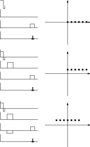
FIGURE 18.29. (a) The signal measured while the x gradient is applied gives the spatial Fourier transform of the image along the kx axis. (b) The addition of a phase-encoding gradient sets a nonzero value for ky so that the readout determines the spatial Fourier transform along a line parallel to the kx axis. (c) Phase encoding along the x axis as well shifts the line along which the coe cients are determined.
values of ky . Application of a gradient Gx during the phase-encoding time (in addition to the readout gradient) changes the starting value of kx. This allows one to determine the coe cients for negative values of kx. This figure has been drawn without taking into account that the application of a π pulse changes kx to −kx and ky to −ky . The gradients and signals for this spin–echo determination are shown in Fig. 18.30. The coe cients are substituted in Eq. 18.47a to reconstruct M (x, y, z) for the z slice in question.
18.9.5Other Pulse Sequences
Dozens of other pulse sequences have been invented, all of which are based on the fundamentals presented here.
532 18. Magnetic Resonance Imaging
π/2 π Bx 


Gz
Gx
Gy
Mx |
FIGURE 18.30. The signals in a standard phase encoding. The pulse sequence is repeated for each value of ky .
|
|
|
π/2 |
|
|
|
|
|
|
|
|
|
|
|
|
|
|
|
|
π |
|
|
|
|
|||||
Bx |
|
|
|
|
|
|
π |
|
|
π |
||||
|
|
|
|
|
|
|
|
|
|
|
|
|
|
|
|
|
|
|
|
|
|
|
|
|
|
|
|
|
|
Gz
Gy
Gx
Mx |
FIGURE 18.31. A fast spin echo sequence uses a single π/2 slice selection pulse followed by multiple echo rephasing pulses. A correction must be made for the transverse decay.
We mention only a few, and there are many variations of these. For details, see Bernstein et al. (2004).
Fast spin echo or turbo spin echo uses a single π/2 pulse, followed by a series of π pulses, as shown in Fig. 18.31. Each π pulse produces an echo, though the echo amplitudes decay and a correction for this must be made in the image reconstruction. Each Gy pulse increments or “winds” the phase by a fixed amount. A negative Gx pulse resets the positions of the kx values. Faster image acquisition sequences not only save time, but they may allow the image to be obtained while the patient’s breath is held, thereby eliminating motion artifacts.
π/2
Bx
Gz
Gy
Gx
Mx |
FIGURE 18.32. Echo planar imaging uses a very uniform magnet and eliminates the rephasing π pulses.
The major problem with conventional spin echo is that one must wait a time TR T1 between measurements for di erent values of ky . One way to speed things up is to use the intervening time to make measurements in a slice at a di erent value of z. Another technique is to use a flip angle smaller than π/2. Suppose the flip angle is α = 20 ◦. This gives a transverse magnetization proportional to sin 20 ◦ = 0.34 while reducing the longitudinal magnetization to cos 20 ◦ = 0.94. Thus, k space can be sampled until the transverse signal has decayed and another α flip pulse can immediately be applied to restore the transverse magnetization.
Echo-planar imaging (EPI) eliminates the π pulses. It requires a magnet with a very uniform magnetic field, so that T2 (in the absence of a gradient) is only slightly greater than T2 . The gradient fields are larger, and the gradient pulse durations shorter, than in conventional imaging. The goal is to complete all the k-space measurements in a time comparable to T2 . In EPI the echoes are not created using π pulses. Instead, they are created by dephasing the spins at di erent positions along the x axis using a Gx gradient, and then reversing that gradient to rephase the spins, as shown in Fig. 18.32. Whenever the integral of Gx(t) is zero, the spins are all in phase and the signal appears. A large negative Gy pulse sets the initial value of ky to be negative; small positive Gy pulses (“blip”) then increase the value of ky for each successive kx readout. Echo-planar imaging requires strong gradients—at least five times those for normal studies— so that the data can be acquired quickly. Moreover, the riseand fall-times of these pulses are short, which induces large voltages in the coils. Eddy currents are also induced in the patient, and it is necessary to keep these below the threshold of sensitivity. These problems can be reduced by using sinusoidally varying gradient currents. Image reconstruction takes longer, because the sample