

Intermediate Physics for Medicine and Biology - Russell K. Hobbie & Bradley J. Roth
.pdf482 17. Nuclear Physics and Nuclear Medicine
TABLE 17.1. Properties of nucleons, the electron, and the neutral hydrogen atom.
Property |
Neutron |
Proton |
Electron |
H atom |
|
Massa |
1.008 664 916 |
1.007 276 47 |
0.000 548 579 9 |
1.007 825 035 |
|
Chargeb |
0 |
+e |
−e |
0 |
|
Rest |
939.565 |
938.272 |
0.5110 |
938.783 |
|
energy |
|
|
|
|
|
m0c2 |
|
|
|
|
|
(MeV) |
≈ 12 min |
|
|
|
|
Half-life |
Stable |
Stable |
Stable |
||
Spin |
1 |
1 |
1 |
. . . |
|
2 |
2 |
2 |
|||
|
|
a1 u is the mass unit; the mass of 12C is 12.000 u by definition; 1 u = 1.660 539 × 10−27 kg.
be = 1.602 177 × 10−19 C.
The final section describes the nuclear decay of radon and some of the considerations in calculating the dose and the risk to the general population. It supplements the material that was introduced in Sec. 16.13.
17.1 Nuclear Systematics
An atomic nucleus is composed of Z protons and N = A − Z neutrons. We call Z the atomic number and A the mass number. Neutrons and protons have very similar properties, as can be seen from Table 17.1. Therefore, they are classed as two di erent charge states of one particle, the nucleon.
Table 17.1 lists the rest mass and the rest energy, the rest mass times the square of the speed of light. One can show using special relativitythat the total energy E of an object with rest mass m0 is related to its speed v and kinetic energy T by
E = |
|
m0c2 |
= m0c2 |
+ T. |
(17.1) |
|
|
− v2 |
/c2)1/2 |
||||
(1 |
|
|
|
|||
In this equation c is the velocity of light. The energy and mass of both the proton and neutral hydrogen atom are given; the distinction will be important later.
It is customary to specify a nucleus by a symbol such as the following for carbon (Z = 6, N = 6, A = 12):
AZ C or 126 C.
The mass number used to be written as a superscript on the right; however, this becomes confusing if the ionization state must also be specified. It is now customary to leave the right side of the symbol for atomic properties. Since the element symbol corresponds to a specific atomic number, Z is often omitted.
Di erent nuclei of the same element with di erent numbers of neutrons are called isotopes. Another isotope of carbon is 11C, which has five neutrons.
The sizes of atoms are roughly constant as one goes through the Periodic Table, with exceptions as shells are filled. On the other hand, the size of nuclei grows steadily
FIGURE 17.1. Plot of atomic radius and nuclear radius vs. atomic number, showing the relative constancy of the atomic radius and the systematic increase of nuclear radius. Shell e ects in atomic radii are quite pronounced; slight shell e ects in the nuclear radius are not shown. Atomic data are from Table 7b–3 of The American Institute of Physics Handbook,
New York, McGraw-Hill, 1957. Nuclear radii are from Eq. 17.2, using the average atomic mass to estimate A from Z.
through the periodic table. The nuclear radius R and atomic mass number are related by
R = R0A1/3. |
(17.2) |
The precise value for R0 depends on how the nuclear radius is measured. If it is measured from the charge distribution, then
R0 = 1.07 × 10⁻¹⁵ m. |
(17.3) |
Figure 17.1 shows how nuclear radii grow systematically, while atomic radii do not change appreciably with A (although they do change dramatically as shells close). The constancy of atomic size results from two competing e ects: as Z increases the outer electrons have a larger value of the principal quantum number n. On the other hand, the greater charge means that Coulomb attraction makes the orbit radius smaller for a given n.
The A1/3 dependence in the nuclear case means that the nuclear density is independent of A. To see this, note that the volume of a spherical nucleus is 4πR3/3 = 4πR03A/3. Since the mass and volume are both proportional to A, the density is constant. This implies that nucleons can get only so close to one another, and that as more are added, the nuclear volume increases. This constant density is the same e ect we see in the aggregation of atoms in a crystal or a drop of water.
17.1 Nuclear Systematics |
483 |
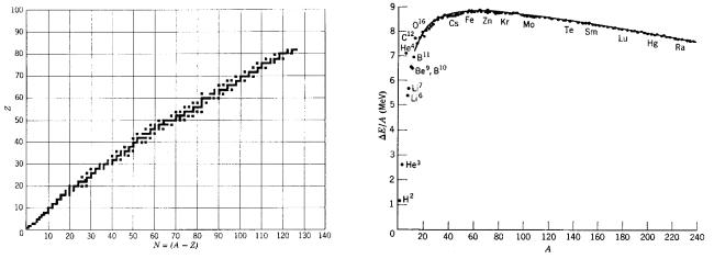
FIGURE 17.2. Stable nuclei. Solid squares represent nuclei which are stable and are found in nature. From Robert Eisberg and Robert Resnick, Quantum Physics of Atoms, Molecules, Solids, Nuclei and Particles, 2nd ed., New York, John Wiley & Sons, 1985, p. 524. Reprinted with permission of John Wiley & Sons.
FIGURE 17.3. The average binding energy per nucleon for stable nuclei. From R. Eisberg and R. Resnick, Quantum Physics of Atoms, Molecules, Solids, Nuclei, and Particles, 2nd ed., New York, John Wiley & Sons, 1985, p. 524. Reprinted with permission of John Wiley & Sons.
Scattering experiments measure the force between two nucleons. At large distances, there is no force between two neutrons or between a neutron and a proton. (Between two protons, of course, there is Coulomb repulsion.) As two nucleons are brought close together, a strong attractive “nuclear” force exists; at still closer distances, the nuclear force becomes repulsive.
If we look at the nuclei that are stable against radioactive decay and are therefore found in nature, we find that for light elements, Z = N . As Z increases, the number of neutrons becomes greater than Z; this can be seen in Fig. 17.2.
Eq. 17.1 shows that when an object is at rest, its total energy (which is its internal energy) is related to its rest mass by
E = m0c2. |
(17.4) |
The measurement of nuclear masses has provided one way to determine nuclear energies. It is necessary to supply energy to a stable nucleus to break it up into its constituent nucleons (or else it would not be stable). The binding energy (BE) of the nucleus is the total energy of the constituent nucleons minus the energy of the nucleus:
BE = Zmpc2 + (A − Z)mnc2 − mnuclc2. (17.5)
It represents the amount of energy that must be added to the nucleus to separate it into its constituent neutrons and protons.
Suppose we add Zmec2 to the first term. Then we have the energy of Z protons plus the energy of Z electrons. Except for the binding energy of each electron, this is the same as the mass of Z neutral hydrogen atoms, which we call Mpc2. Similarly, we can add the mass of Z electrons to mnuclc2 and neglect the electron binding energy to obtain Matomc2. Capital M represents the mass of a
neutral atom, while m stands for the mass of a bare nucleus. For the neutron, m = M . In Eq. 17.5, we can add Zmec2 to the first term and add Zmec2 to the last term, to obtain the binding energy in terms of the masses of the corresponding neutral particles:
BE = ZMpc2 + (A − Z)Mnc2 − Matomc2. (17.6)
This is fortunate, because neutral masses (or those for ions carrying one or two charges) are the quantities actually measured in mass spectroscopy.
Masses are measured in unified mass units u, defined so that the mass of neutral 12C is exactly 12 u. Carbon is used for the standard because hydrocarbons can be made in combinations to give masses close to any desired mass. The carbon standard replaced one based on the naturally occurring mixture of oxygen isotopes in the early 1960s. (One of the troubles with the earlier standard was that the relative abundance of the various oxygen isotopes varies with time and with location on the earth.) The earlier unit was called the atomic mass unit, amu. One still finds confusion in the literature about which standard is being used, and the carbon standard is sometimes called an amu.
One unified mass unit is related to the kilogram, the joule, and the electron volt by
1 u = 1.660 54 × 10−27 kg, |
|
|
(1 u)(c2) = $ |
1.492 41 × 10−10 J |
(17.7) |
|
931.49 MeV. |
|
If one plots the binding energy per nucleon versus mass number as in Fig. 17.3, one sees that the binding energy per nucleon has a maximum near A = 60, and that the average binding energy (except for light elements) is about 8 MeV per nucleon. For less stable nuclei on either side of the stable line plotted in Fig. 17.2, the binding energy is less than that for the nuclei shown here.

484 17. Nuclear Physics and Nuclear Medicine
The maximum near A = 60 is what makes both fission and fusion possible sources of energy. A heavy nucleus with A near 240 can split roughly in half, giving two fission products. Since the nucleons in each of the products are more tightly bound on the average than in the original nucleus, energy is released. This energy di erence comes almost entirely from the Z2 dependence of the Coulomb repulsion of the protons in the nuclei. In fusion, two nuclei of very low A combine to give a nucleus of higher A, for which the binding energy per nucleon is greater.
17.2Nuclear Decay: Decay Rate and Half-Life
If a nucleus has more energy than it would if it were in its ground state, it can decay. If the nucleus has su - cient energy, it can emit a proton, neutron, or cluster of nucleons [α particle (42He), deuteron (21H), etc.]. When a nucleus has enough excitation energy to decay by nuclear emission it usually does so in such an extremely short time that the nuclei could never be introduced in the body after they were produced. An exception is the α decay of a few elements near the upper (high-Z) end of the periodic table. They are found in nature, either because their lifetimes are very long or because they are formed as the result of some other decay process that has a long lifetime.
If a nucleus has just a small amount of excess energy, it emits a γ ray, a photon analogous to the x ray or visible photons emitted by an excited atom. Another process that can occur is the emission of a positive or negative electron, with the conversion of a proton to a neutron, or vice versa. This is called β decay. Both γ and β decay will be described in detail in the next two sections.
Each excited nucleus has a probability λ dt of decaying in time dt. When there are N nuclei present, the average number decaying in time dt is1
−dN = N λ dt.
The rate of change of N is the activity, A(t), the number of decays per second:
A(t) = dNdt = −λN.
This leads to the familiar exponential decay of Chapter
2:
N = N0e−λt.
The half-life T1/2 is related to λ by Eq. 2.10:
T1/2 = |
0.693 |
. |
(17.8) |
|
|||
|
λ |
|
|
1The decay constant is called λ in this chapter to conform to the usage in nuclear medicine.
17.3Gamma Decay and Internal Conversion
When a nucleus is in an excited state, it can lose energy by photon emission. The energy levels of the nucleus are characterized by certain quantum numbers, and γ emission is subject to selection rules analogous to those for x-ray emission by atoms. Half-lives for γ emission range from 10−20 to 10+8 s.
Figure 17.4 shows an energy level diagram for 9943Tc (technetium), an isotope widely used in nuclear medicine, along with some tabular material that we will need as we progress through this chapter. There are two important levels to consider in 9943Tc. The ground state is not stable but decays by β decay, considered in the next section. However, its decay rate is so small (half-life of 2.12 × 10⁵ years) that we can ignore its decay. There is a level at an excitation of 0.143 MeV above the ground state that has a half-life of 6 h for γ decay. This is an unusually long half-life; we call it a metastable state and denote it by 99mTc. Looking at the table labeled input data, we see that there are two modes of decay of the nucleus from this state. The first is the emission of a 0.0021-MeV γ ray followed by a 0.1405-MeV γ ray. It occurs 0.986 of the time. The other possibility is the emission of one γ ray, of energy 0.1426 MeV, which happens in 0.014 of the decays.
The notations E3, M 1, and M 4 in the last column of the input data refer to the selection rules and quantum number changes in the transitions. We will not need the details, although they can be used to estimate the decay rates. The labels E1, E2, and E3 are called electric dipole, electric quadrupole, and electric octupole, respectively. M 1 means magnetic dipole, and M 4 means magnetic 24 or magnetic hexadecapole.
Whenever a nucleus loses energy by γ decay, there is a competing process called internal conversion. The energy to be lost in the transition, Eγ , is transferred directly to a bound electron (usually a K or L electron), which is
then ejected with a kinetic energy |
|
T = Eγ − B, |
(17.9) |
where B is the binding energy of the electron.
The mean number per disintegration in the table of input data is the mean number of times that the indicated transition between energy levels takes place. In the table of output data, on the other hand, it means the mean number of times that radiation is emitted. To see the distinction, compare the γ2 entries in the input data and output data of Fig. 17.4. The γ2 transition from the 0.1405-MeV level to the ground state occurs 0.9860 times per disintegration. From the output data, we see that this transition takes place by emission of a photon (γ2) 0.8787 times, by K internal conversion 0.0913 times, by L internal conversion 0.0118 times, and by M internal conversion 0.0039 times (the sum is 0.9857, which agrees with the value 0.9860 times per disintegration).
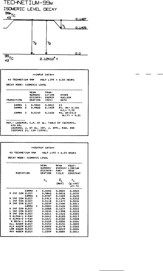
FIGURE 17.4. Energy levels and decay data for the isotope 99mTc. The various features are discussed in the text. Reprinted by permission of the Society of Nuclear Medicine from Dillman, L. T., and F. C. Von der Lage. MIRD Pamphlet No. 10. Radionuclide Decay Schemes and Nuclear Parameters for Use in Radiation Dose Estimation, 1974, p. 62.
17.4 Beta Decay and Electron Capture |
485 |
To calculate the mean number of times a radiation is emitted from the mean number of transitions, we need numbers f that are the fraction of transitions involving a particular radiation. The fraction associated with γ decay is fr , the fraction with K internal conversion is fK , and so forth. The sum of all these fractions is unity:
fr + fK + fL + fM + · · · = 1. |
(17.10) |
Often these fractions are not listed in the literature. Instead, one finds the internal conversion coe cient α. For conversion of a K electron, it is αK = fK /fr . For the L shell it is αL = fL/fr , and so on. One also finds in the literature the ratio
K = fK = αK .
L fL αL
A useful empirical relationship is that fM ≈ fL/3. In the input data of Fig. 17.4, αK is called AK.
Once internal conversion has created a hole in the electronic structure of the atom, characteristic x rays and Auger electrons will be emitted. They must also be considered in calculating the total dose from the nuclear decay.
17.4 Beta Decay and Electron Capture
Nuclei that are not on the line of stability in Fig. 17.2 have greater internal energy and are susceptible to some kind of decay. They can lose energy by γ emission. In addition, nuclei above the line of stability have too many protons relative to the number of neutrons; nuclei below the line have relatively too many neutrons.
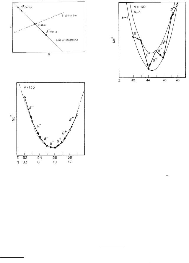
Two modes of decay allow a nucleus to approach the stable line. In beta (β− or electron) decay, a neutron is converted into a proton. This keeps A constant, lowering N by one and raising Z by one. In positron (β+) decay, a proton is converted into a neutron. Again A remains unchanged, Z decreases and N increases by 1. We find β+ decay for nuclei above the line of stability and β− decay for nuclei below the line. Figure 17.5 shows a portion of the line of stability, a line of constant A (Z = A − N ), and the regions for β+ and β− decay.
We can plot the energy of the neutral atom for di erent nuclei along the line of constant A. Since there are one or two stable nuclei, there is some value of Z and N for which the energy is a minimum. The energy increases in either direction from this minimum. The first approximation to a curve with a minimum is a parabola, as shown in Fig. 17.6 for a nucleus of odd A.2 When Z is too small, a neutron is converted to a proton by β− decay. If Z is too large, a proton changes to a neutron by β+ decay or electron capture (to be described below).
2This parabola and the general behavior of the binding energy with Z and A can be explained remarkably well by the semiempir-
486 17. Nuclear Physics and Nuclear Medicine
FIGURE 17.5. β− decay and β+ decay do not change A. They do change N and Z to bring the nucleus closer to the stability line.
FIGURE 17.6. Energy of nuclei as a function of Z for an odd value of A (A = 135). The only stable nucleus is 13556 Ba; nuclei of lower Z undergo β− emission; those of higher Z undergo β+ emission or electron capture.
When A is odd, there are an even number of protons and an odd number of neutrons (even–odd) or vice versa (odd–even). When we plot the energies of even-A nuclei, we find that the masses lie on two di erent parabolas (Fig. 17.7). The one for which both Z and N are odd (odd–odd) has greater energy than the parabola for which both are even. The reason is that nucleons have lower energy when they are paired with one another in such a way that their spins are antiparallel. In the even–even case, the neutrons and the protons are all paired o and have this lower energy; in the odd–odd case there are both an unpaired proton and an unpaired neutron, and the en-
ical mass formula [Evans (1955, Chapter 11); Eisberg and Resnick, (1985, p. 528)].
FIGURE 17.7. Energy of even-A nuclei as a function of Z. Nuclei with an odd number of protons and neutrons have higher energies than those with an even number of each. This makes it possible for the same nucleus to decay by either β− or β+ emission.
ergy is higher. As we change Z by one, we jump back and forth between the odd–odd and the even–even parabolas. For odd-A nuclei, either the neutrons are paired and one proton is not, or vice versa. There is always one unpaired nucleon as Z changes, so there is only one parabola.
The existence of the two parabolas means that there are usually (but not always) two stable nuclei with an odd–odd nucleus between them that can decay by either β− or β+ emission.
The emission of a β− particle is accompanied by the emission of a neutrino (strictly speaking, an antineu-
trino): |
|
ZAX →ZA+1 Y + β− + ν. |
(17.11) |
The neutrino has no charge and no rest mass,3 so that like a photon, it travels with velocity c and its energy and momentum are related by E = pc. Neutrinos hardly interact with matter at all, so they are quite di cult to detect. Nevertheless they have been detected through certain specific nuclear reactions that take place on the rare occasions when a neutrino does interact with a nucleus. A particle that seemed originally to be an invention to conserve energy and angular momentum now has a strong experimental basis.
Suppose that β decay consisted of the ejection of only a β particle. If the original nucleus X were at rest,4 then nucleus Y would recoil in the direction opposite the β
3Recent measurements indicate that the neutrino may have a rest mass, but it is less than 3 eV. [S. Eidelman et al. (Particle Data Group), Phys. Lett. B 592: 1 (2004) (URL: http://pdg.lbl.gov)]
4Its thermal energy of about 401 eV is negligible compared to the energy released in decay.
17.4 Beta Decay and Electron Capture |
487 |
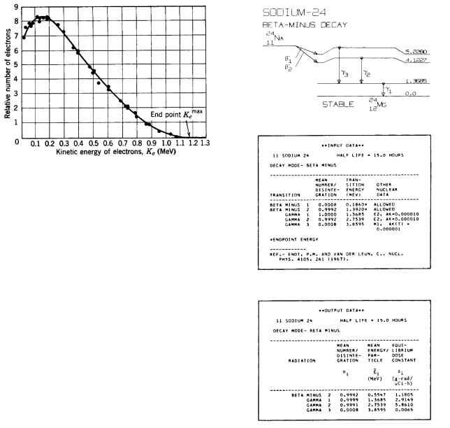
FIGURE 17.8. A typical spectrum of β particles. In this case it is for the β decay of 21083 Bi. From Robert Eisberg and Robert
Resnick. Quantum Physics of Atoms, Molecules, Solids, Nuclei, and Particles, 2nd ed., p. 566. Copyright c 1985 John Wiley & Sons. Reproduced by permission of John Wiley & Sons.
particle to conserve momentum; the ratio of its velocity to that of the β particle would be given by their mass ratio. The recoil nucleus and the β particle would each have a definite fraction of the total energy available from the decay, and the β particles would all have the same energy. However, the observed β-particle energy spectrum is not a line spectrum but a continuum ranging from zero to the expected energy, as shown in Fig. 17.8. The missing energy is carried by the neutrino. The di erent energies correspond to di erent angles of emission of the neutrino relative to the direction of the β particle. This kind of spectrum is characteristic of three bodies emerging from the reaction.
The total kinetic energy for the three emerging particles is
Edecay = mZ,Ac2 − mZ+1,Ac2 − mec2.
If we add and subtract Zmec2, the result is unchanged:
Edecay = (mZ,Ac2 + Zmec2) − (mZ+1,Ac2 (17.12)
+Zmec2 + mec2)
=MZ,Ac2 − MZ+1,Ac2.
FIGURE 17.9. Energy levels and data for the β decay of 24Na. Reprinted by permission of the Society of Nuclear Medicine from L. T. Dillman and F. C. Von der Lage. MIRD Pamphlet No. 10. Radionuclide Decay Schemes and Nuclear Parameters for Use in Radiation Dose Estimation, p. 19.
The energy released in the decay is given by the di erence in rest energies of the initial and final neutral atoms. This energy is shared in di erent amounts by the three particles; it is shared mainly by the neutrino and electron, since the nucleus is so massive and its kinetic energy is p2/2m. The maximum or end-point energy of the β spectrum in Fig. 17.8 corresponds to Edecay.
Figure 17.9 shows data for the decay of 24Na, an isotope that has been used in nuclear medicine. The transition labeled β2 is overwhelmingly the most common. The β2 emission is followed by two γ rays, and the end-point energy of the β decay is 1.392 MeV. On the other hand,
the average energy of the β particle is only 0.5547 MeV, about 40% of the end-point energy.
Emission of a positron converts a proton into a neutron, and Z decreases by one. A neutrino is also emitted:
ZAX →ZA−1 Y + β+ + ν. |
(17.13) |
The decay energy is again given by
Edecay = mZ,Ac2 − mZ−1,Ac2 − mec2.
However, this time, when we add Zmec2 to the first term and subtract (Z −1)mec2 from the second term to convert
488 17. Nuclear Physics and Nuclear Medicine
nucleus (we ignore its kinetic energy): |
|
Ee.c. = mec2 + mZ,Ac2 − mZ−1,Ac2. |
|
If we add and subtract (Z − 1)mec2, we have |
|
Ee.c. = MZ,Ac2 − MZ−1,Ac2. |
(17.15) |
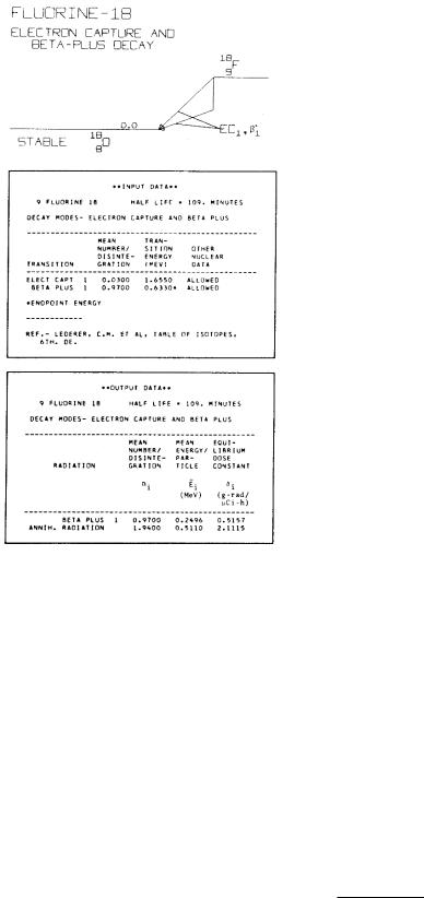
A K electron5 is usually captured. The energy from the nuclear transition is given to a neutrino. No electron emerges, but there are K x rays and Auger electrons,6 as there are any time a vacancy in the K shell occurs, and these contribute to the radiation dose. They are not listed in the output data of Fig. 17.10 because the K x rays only have an energy of about 530 eV. We now understand that Auger electrons can be very important in the dose in some cases.
There is also an entry under output data labeled annihilation radiation. Once a positron has been emitted, it slows down like any other charged particle. At some point it combines with an electron (since the positron and electron constitute a particle–antiparticle pair), and all of the rest energy of both particles goes into two photons.7 The energy conservation equation is
2mec2 = 2hν. |
(17.16) |
For each original positron emitted, two photons are produced, each of energy mec2 = 0.511 MeV.
FIGURE 17.10. Energy levels and data for the β+ decay of 18F. Reprinted by permission of the Society of Nuclear Medicine from L. T. Dillman and F. C. Von der Lage. MIRD Pamphlet No. 10. Radionuclide Decay Schemes and Nuclear Parameters for Use in Radiation Dose Estimation p. 18.
these to atomic masses, the electron masses do not cancel. Instead, we get
Edecay = MZ,Ac2 − MZ−1,Ac2 − 2mec2. (17.14)
Positron emission will not occur unless the initial neutral atomic mass exceeds the final neutral atomic mass by at least 2mec2. We remind ourselves of this by drawing a vertical line of length 2mec2 before drawing the slanting line for the β+ decay, as in Fig. 17.10, the decay scheme for 18F.
The first entry in the table of input data in Fig. 17.10 is for electron capture. The transition energy listed is 2mec2 more than for β+ decay. Some of the inner electrons of the atom are close enough to the nucleus (quantummechanically, the electron wave functions overlap the nucleus enough) so that the electron is captured by the nucleus, and a neutrino is emitted. In terms of nuclear masses, an electron rest energy is added to the parent
17.5Calculating the Absorbed Dose from Radioactive Nuclei within the Body
When a radiopharmaceutical is given to a patient for either diagnosis or therapy, the nuclei end up in di erent organs in varying amounts; for example, 99mTc-labeled albumin microspheres injected intravenously lodge in the lungs. The problem is to calculate the whole-body absorbed dose, the dose to the lungs, and the dose to other organs.
The dose calculation is carried out in the following way:8
1. Calculate the total number of nuclear transformations or disintegrations in organ h. It is called the
˜
cumulated activity Ah or Nh.
2.Calculate the mean energy emitted per unit cumulated activity for each type of photon or particle emitted.
5See Chapter 14.
6See Chapter 14.
7Three photons are occasionally emitted.
8Dose calculations in this chapter follow the technique and notation recommended by the MIRD Committee of the Society of Nuclear Medicine [Loevinger et al. (1988) and Stabin et al. (2005)].

(a)If the radioactive nucleus can emit several types of particles or photons per transformation, call ni the mean number of particles or photons of type i emitted per transformation. These include γ rays, electrons, x rays and Auger electrons. [In the “output data” of Dillman and Von der Lage (1974), ni is called the mean number per disintegration. In the more recent report of Weber et al. (1989) it is called particles per transition. We have continued to show the older tables here because the newer ones contain only the output data.] The data are also available in electronic form [Eckerman et al. (1994); Stabin and da Luz (2002); RADAR (the Radiation Group Assessment Resource), www.doseinfo-radar.com; and the National Nuclear Data Center, www.nndc.bnl.gov/mird/].
(b)For each type i determine Ei, the mean energy per particle or photon.
(c)Calculate ∆i = niEi, the mean energy emitted per unit cumulated activity, for each type of particle or photon emitted. (In earlier MIRD literature, this was called the equilibrium absorbed dose constant.)
3.Calculate φi(rk ← rh), the fraction of the radiation of type i emitted in source region rh that is absorbed in target region rk , and divide by the mass of the target region to get the specific absorbed fraction
Φi(rk ← rh) = φi(rk ← rh) . mk
(Φ has the units of inverse mass.)
4.The mean absorbed dose in organ k due to activity in organ h, D (in J kg−1 or Gy) is
|
|
(rk ← rh) = A˜h i niEiΦi(rk ← rh), |
|
|
D |
(17.17) |
|||
|
|
(rk ← rh) = A˜h i ∆iΦi(rk ← rh). |
|
|
|
D |
|
||
5.If several organs are radioactive, a sum must be taken over each organ:
D |
(rk ) = |
A˜h |
i |
∆iΦi(rk |
← |
rh). (17.18) |
|
|
h |
|
|
˜
The next three sections show how to determine A, ∆i, and Φi. Some tables [Snyder et al. (1969, 1976)] give values of Φi for photons of various energies. It is necessary to multiply by ∆i and sum for the isotope of interest. These sums must be repeated over and over again for common radionuclides. The sum is called the mean absorbed dose per unit cumulated activity:
S(rk |
← |
rh) = |
∆iΦi(rk |
← |
rh), |
(17.19) |
||
|
|
|
|
i |
|
|
||
|
|
|
|
|
˜ |
|
|
(17.20) |
|
|
|
|
|
|
|
||
D(rk ← rh) = AhS(rk ← rh), |
||||||||
17.6 Activity and Cumulated Activity |
489 |
D(rk ) = h ˜hS(rk ← rh). (17.21)
A
A table of S for many common radionuclides is available [Snyder et al. (1975)]. The tables cannot be
˜
summed over h because the values of Ah depend on how the isotope is administered. A computer program OLINDA/EXM is most commonly used for these calculations [Stabin, Sparks and Crowe (2005)]. These authors call S the dose factor.
To discuss units, imagine there is only one type of ra-
diation. In SI units the dose is simply |
|
|
|
||
|
˜ |
|
|
1 |
|
D (Gy) = |
A (dimensionless) |
[∆i (J)] |
Φi (kg− |
|
) . |
(17.22a) In day-to-day calculations, it is often easier to use mixed units and write
|
Gy kg |
˜ |
|
D(Gy) = k |
|
A (MBq s) |
(17.22b) |
|
|||
|
MBq s MeV |
|
|
×[∆i (MeV)] Φi (kg−1)
In an older system of units, where the dose is in rad and the total number of transitions is in microcurie-hour (see below), the equation is
|
˜ |
|
1 |
1 |
|
Φi (g− |
1 |
|
D(rad) = |
A (µCi h) |
∆i (g rad µCi− |
|
h− |
) |
|
) . |
(17.22c) The next three sections discuss cumulated activity, the mean energy emitted, and the absorbed fraction of the energy. Then all of these concepts are combined with ex-
amples of absorbed dose calculations.
17.6 Activity and Cumulated Activity
The activity A(t) is the number of radioactive transitions (or transformations or disintegrations) per second. The SI unit of activity is the becquerel (Bq):
1 Bq = 1 transition s−1. |
(17.23) |
The earlier unit of activity, which is still used occasionally, is the curie (Ci):
1 Ci = 3.7 × 10 |
10 |
Bq, |
(17.24) |
4 |
|||
1 µCi = 3.7 × 10 |
Bq. |
|
|
˜
The cumulated activity A is the total number of transitions that take place. The SI unit of cumulated activity is the transition or the Bq s. Both are dimensionless. The old unit of cumulated activity is the µCi h:
1 µCi h = 1.332 × 10⁸ Bq s. |
(17.25) |
Consider a sample of N0 radioactive nuclei |
at time |
t = 0. The total number of nuclei remaining at time t is N (t) = N0e−λt, and the total activity is A(t) = λN (t) =
490 17. Nuclear Physics and Nuclear Medicine
A0e−λt. The cumulated activity between times t1 is
A˜(t1, t2) = |
t2 |
A(t) dt = |
A0 |
e− |
λt |
− e− |
λt |
|
|
|
1 |
2 |
|||||
t1 |
λ |
= N (t1) − N (t2).
If all times are considered, t1 = 0 and t2 = ∞,
˜ |
˜ |
A0 |
|
A0T1/2 |
|
|
A |
= A(0, ∞) = |
λ |
= |
|
0.693 |
= 1.443A0T1/2. |
This is, as we would expect, N0.
and t2
(17.26)
(17.27)
and elsewhere [Loevinger et al. (1988), p. 23]. The activity in the organ is Ah(t) = Ahe−λt. [Note the di erence between the activity in organ h as a function of time, Ah(t), the initial activity in organ h, Ah, and the cumu-
˜
lated activity in organ h, Nh = Ah.] Let the fraction of
the activity in the organ be Fh. The cumulated activity is
A˜h = Ah ∞ e−λt dt = |
Ah |
= |
FhA0 |
. |
||||
λ |
|
|||||||
|
0 |
|
|
|
λ |
|||
The residence time is |
|
|
|
|
|
|
||
|
˜ |
Fh |
|
|
|
|
|
|
τh = |
Ah |
= |
= 1.443FhT1/2. |
(17.31) |
||||
|
λ |
|||||||
|
A0 |
|
|
|
|
|
||
17.6.1The General Distribution Problem: Residence Time
Suppose that a radioactive substance is introduced in the body by breathing, ingestion, or injection. It may move into and out of many organs before decaying, and it may even leave the body. The details of how it moves depend on the pharmaceutical to which it is attached.
The cumulated activity in organ h is the total number of disintegrations in that organ:
˜ |
∞ |
(17.28) |
Nh = Ah = |
Ah(t) dt. |
|
|
0 |
|
The dose is to organ k is then
Dk = |
NhS(rk |
← |
rh). |
(17.29) |
|
h |
|
|
The units of Nh are disintegrations (dimensionless) or Bq s. If initial activity A0 (Bq) is administered to the patient, the ratio Nh/A0 is called the residence time in organ h:
|
Nh |
|
˜ |
|
|
˜ |
|
|
|
τh = |
= |
Ah |
= |
Ah(0, |
∞) |
. |
(17.30) |
||
A0 |
A0 |
|
A0 |
|
|||||
|
|
|
|
|
|
|
|||
The residence time is the length of time that activity at a constant rate A0 would have to reside in the organ to give that cumulated activity. The residence time for a given substance and organ must be determined by measurement, guided by the use of appropriate models. Many residence times have been determined and published. The presence of an abnormality in some organ can drastically alter the residence time.
We now calculate the cumulated activity and residence time for some simple situations.
17.6.2Immediate Uptake with No Biological Excretion
This is the simplest example. A certain fraction of the radiopharmaceutical is taken up very rapidly in some organ, and it stays there. This is a good model for 99mTc– sulfur colloid, which is used for liver imaging. About 85% is trapped in the liver; the remainder goes to the spleen
17.6.3Immediate Uptake with Exponential Biological Excretion
Suppose that in addition to physical decay with decay constant λ, the pharmaceutical moves to another organ while it is still radioactive. Such a process can be complicated, perhaps involving storage in the gut or bladder. In other cases, the disappearance from a particular organ may be close to exponential with a biological disappearance constant λj . (Assume for now that all the radioactive nuclei can disappear biologically. If some are bound in di erent chemical forms, this might not be true.) If N is the number of radioactive nuclei in the organ (not the total number originally administered), then the rate of change of N is
dN
dt = −(λ + λj )N,
the solution to which is N (t) = N0e−(λ+λj )t. The activity is λN , not −dN /dt. Since it is proportional to N , we can again write
Ah(t) = Ahe−(λ+λj )t = λN0e−(λ+λj )t. |
(17.32) |
Again, N0 = Ah/λ. The decay constant λ + λj is larger than the physical decay constant. The e ective half-life is
(Tj ) = 0.693 . (17.33)
e |
λ + λj |
|
In terms of the physical and biological half-lives T and Tj , this is
|
|
1 |
|
= |
|
1 |
+ |
1 |
|
(17.34) |
|||||
|
|
(Tj ) |
e |
|
T |
Tj |
|||||||||
|
|
|
|
|
|
|
|||||||||
or |
|
|
|
|
|
|
|
|
|
|
|
|
|
|
|
|
|
|
|
|
|
|
|
T Tj |
|
|
|
|
|||
|
|
(Tj ) |
|
= |
|
|
|
|
. |
(17.35) |
|||||
|
e |
|
|
|
|
|
|
|
|||||||
|
|
|
|
|
|
T + Tj |
|
||||||||
|
|
|
|
|
|
|
|
||||||||
The cumulated activity is |
|
|
|
|
|
|
|
|
|
|
|
||||
|
|
|
|
t2 |
|
|
|
|
|
|
|
|
|
|
|
A˜h(t1, t2) = Ah |
|
e−(λ+λj )t dt |
(17.36) |
||||||||||||
|
Ah |
|
|
|
t1 |
|
|
|
|
|
|
|
|
|
|
= |
e−(λ+λj )t1 |
− |
e−(λ+λj )t2 . |
|
|||||||||||
|
λ + λj |
|
|
|
|
|
|
|
|
|
|
|
|||
|
2.0 |
|
|
|
|
|
1.5 |
|
|
|
|
|
|
2e-2t |
|
|
|
0 |
1.0 |
|
|
|
|
N/N |
|
|
|
|
|
|
|
|
|
|
|
|
N1 = e-3t |
|
|
|
|
|
0.5 |
|
|
|
|
|
|
N2 = 2(e-2t - e-3t ) |
|
|
|
|
0.0 |
0.5 |
1.0 |
1.5 |
2.0 |
|
0.0 |
||||
|
|
|
t |
|
|
|
2 |
|
|
|
|
|
1 |
2e-2t |
|
|
|
|
6 |
|
|
|
|
|
5 |
|
|
|
|
|
4 |
|
|
|
|
|
3 |
|
|
|
|
0 |
2 |
|
N2 = 2(e-2t - e-3t ) |
|
|
N/N |
0.1 |
|
|
|
|
|
|
|
|
|
|
|
6 |
|
-3t |
|
|
|
|
N1 = e |
|
|
|
|
5 |
|
|
|
|
|
|
|
|
|
|
|
4 |
|
|
|
|
|
3 |
|
|
|
|
|
2 |
|
|
|
|
|
0.01 |
0.5 |
1.0 |
1.5 |
2.0 |
|
0.0 |
||||
|
|
|
t |
|
|
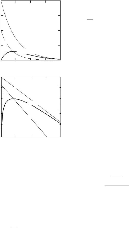
FIGURE 17.11. An example of two-compartment transfer when λ = 1, λ1 = 2, and λ2 = 1.
The cumulated activity for all time is
˜ |
Ah |
|
|
|
Ah = |
λ + λj |
= 1.443 (Tj )e |
Ah. |
(17.37) |
|
|
|
|
17.6.4Immediate Uptake Moving through Two Compartments
Consider the simplest two-compartment model. A total of N0 nuclei are administered that move immediately to the first compartment. They then move exponentially from the first compartment to the second but do not move back. The number in the first compartment is given by
dN1 |
= −(λ1 + λ)N1. |
(17.38) |
dt |
17.6 Activity and Cumulated Activity |
491 |
The radioactive decay constant is λ and the biological disappearance rate is λ1. In compartment 2, the substance enters from compartment 1 and is biologically removed with constant λ2:
dN2 |
= +λ1N1 − (λ + λ2)N2. |
(17.39) |
dt |
Suppose we start with no nuclei in either compartment and inject N0 nuclei in compartment 1 at t = 0. Then one can show (see Problem 11) that
|
|
|
N1(t) = N0e−(λ+λ1)t |
(17.40) |
|||||
so |
|
|
|
|
|
|
|
|
|
|
dN2 |
= λ1N0e−(λ+λ1)t − (λ + λ2)N2, |
(17.41) |
||||||
|
dt |
||||||||
the solution to which is |
|
|
|
|
|
||||
N2(t) = N0 |
λ1 |
|
(λ+λ2)t |
|
(λ+λ1)t |
|
|||
|
|
e− |
|
− e− |
|
. (17.42) |
|||
λ1 − λ2 |
|
|
|||||||
These solutions are worth examining. They are plotted in Fig. 17.11 for λ = 1, λ1 = 2, and λ2 = 1. The number of nuclei in compartment 1 is N0e−3t. At first, many of the particles leaving compartment 1 enter compartment 2, and N2 rises. When there is no more of the substance entering the second compartment from the first, N2 decays at a rate λ + λ2 = 2. This corresponds to the vanishing of the second term in Eq. 17.42. The larger the value of λ1, the faster the second term vanishes. For very large values of λ1, the second term vanishes quickly, the factor λ1/(λ1 − λ2) approaches unity, and the decay is nearly N2(t) = N0e−(λ+λ2)t. The case λ1 = λ2 is discussed in Problem 13. The activities are
A1(t) = λN1(t), A2(t) = λN2(t)
and the cumulated activities are obtained by integration:
|
˜ |
= |
A0 |
|
|
|
|
A1 |
λ + λ1 |
, |
|
||
˜ |
|
|
|
A0λ1 |
(17.43) |
|
= |
|
|
|
|
||
A2 |
|
. |
||||
(λ + λ1)(λ + λ2) |
||||||
The residence times are
1
τ1 = λ + λ1 ,
λ1
(17.44)
τ2 = (λ + λ1)(λ + λ2) .
17.6.5More Complicated Situations
A number of more complicated situations are solved by Loevinger et al. (1988). These include situations where substances move between compartments in both directions, the experimental data for the activity have been fit with a series of exponentials, and convolution techniques are used. All of these cases are for isotopes and pharmaceuticals used in clinical practice.