Intermediate Physics for Medicine and Biology - Russell K. Hobbie & Bradley J. Roth

360 14. Atoms and Light

explained by assuming that light consists of an electromagnetic wave. By an electromagnetic wave, we mean that

1.Light can be produced by accelerating an electric charge.

2.Light has an electric and a magnetic field associated with it; the force that the light exerts on a charged particle is given by Eq. 8.2, F = q(E + v × B). The force due to the magnetic field is usually very small.

3.The velocity of light traveling in a vacuum is given by electromagnetic theory as c = 1/√ 0µ0, where parameters 0 and µ0 are measured in the laboratory for “ordinary” electric and magnetic fields.

In the early twentieth century, light was discovered to have both particle properties and electromagnetic wave properties at the same time. This rather disconcerting discovery was followed a few years later by the discovery that matter, which had been thought to consist of particles, also has wave properties.

A traveling wave of light can be described by a function of the form f (x − cnt), which represents a disturbance traveling along the x axis in the positive direction. (To keep a particular value for the argument of f constant, x must increase as time increases.) If the wave is sinusoidal, then the period, T , frequency, ν,1 and wavelength, λ, are

As light moves from one medium into another where it travels with a di erent speed, the frequency remains the same. The wavelength changes as the speed changes.

Each particle of light or photon has energy E. The energy of each photon (a “particle” concept) is related to

The proportionality constant h is called Planck’s constant. It has the numerical value2

1We used f for frequency in earlier chapters because this is customary when discussing noise. Here we adopt ν for frequency, the notation most often used in atomic physics.

2The electron volt (eV) is a unit of energy. 1 eV= 1.6 × 10−19 J. It is the energy acquired by an electron that moves through a potential di erence of 1 V.

TABLE 14.1. The regions of the electromagnetic spectrum and their boundaries

The electromagnetic spectrum includes radio waves; microwaves, infrared, visible, and ultraviolet light; x rays; and gamma rays. Table 14.1 shows the wavelengths that separate these arbitrary regions, together with the frequencies and the energies of the photons. Visible-light photons have an energy of a few electron volts. X rays are 104–107 times more energetic, while γ rays, which come from atomic nuclei, are often even more energetic but may have energies overlapping x-ray energies. The only di erence between x rays and γ rays is their source.

The property of light that we associate with color is the frequency or the energy of each photon. Visible light covers a narrow range of frequencies, about an octave (a factor of 2). Table 14.2 shows the wavelengths and

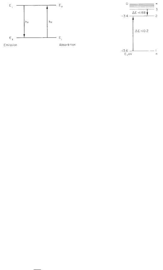
FIGURE 14.1. A system can change from one energy to another by emitting or absorbing a photon. The photon has an energy equal to the di erence in energies of the two levels.

frequencies dividing the colors of the visible spectrum. The frequencies are in the 400–750 THz range.

Most of the e ects discussed in this chapter can be explained by assuming that light is made up of photons.

14.2Atomic Energy Levels and Atomic Spectra

The simplest system that can emit or absorb light is an isolated atom. An atom is isolated if it is in a monatomic gas. In addition to translational kinetic energy, isolated atoms have specific discrete internal energies, called energy levels. An atom can change from one energy level to another by emitting or absorbing a photon with an energy equal to the energy di erence between the levels. Let the energy levels be labeled by i = 1, 2, 3, ..., with the energy of the ith state being Ei. There is a lowest possible internal energy for the atom; when the atom is in this state, no further energy loss can take place. If Ei is greater than the lowest energy, then the atom can lose energy by emitting a photon of energy Ei − Ef and exist in a lower-energy state Ef (Fig. 14.1).

It is possible, using techniques of quantum mechanics, to calculate the energies of the levels with reasonable accuracy (and in some cases with spectacular accuracy). For our purposes, we need only recognize that energy levels exist and know their approximate values. You may be familiar with the hydrogen atom, in which the energy of the nth level is given by

The energy is in joules when the electron mass me is in kilograms, the electronic charge e is in coulombs, and is in J s. The Coulomb’s law constant 1/4π 0 is given in Eq. 6.2. Dividing the energy in joules by e gives the energy in electron volts:

FIGURE 14.3. The spectrum for hydrogen plotted vs. wavelength and the energy levels for hydrogen. Some spectral lines and the corresponding transitions have been labeled.

FIGURE 14.4. A diatomic molecule. Vectors r1 and r2 are the positions of the atoms measured in the laboratory. Vectors R1 and R2 are coordinates in the center-of-mass system. Vector r is the position of the center of mass.

rid of this excess energy by radiating a photon, with the excited electron falling to an unoccupied state with lower energy. This change is usually consistent with the following selection rules, which can be derived using quantum mechanics:

dom and the spin associated with ms. The internal energy of the atom is the sum of the kinetic and potential energies of each electron. The energy of each electron depends on the values of its quantum numbers. It is influenced by the electric field generated by the nucleus and all the other electrons. There are also magnetic interactions between electrons and between each electron and the nucleus, because the moving charges generate magnetic fields.

No two electrons in an atom can have the same values for all their quantum numbers, a fact known as the Pauli exclusion principle.

The ionization energy is the smallest amount of energy required to remove an electron from the atom when the atom is in its ground state. For hydrogen the ionization energy is 13.6 eV. In contrast, it takes only 5.1 eV to remove the least-tightly-bound electron from a sodium atom.

An atom can receive energy from an external source, such as a collision with another atom or some other particle. It can also absorb a photon of the proper energy. Absorbing just the right amount of energy allows one of its electrons to move to a higher energy level, as long as that level is not already occupied. The atom can then get

14.3 Molecular Energy Levels

In addition to internal energy, an atom can have kinetic energy of translation with three degrees of freedom. The translational kinetic energy is also quantized, but as long as the atom is not confined to a very small volume, the levels are so closely spaced that the translational kinetic energy can be regarded as continuous.

Two atoms together have six degrees of translational freedom, because each can move in three-dimensional space. However, if the atoms are bound together, their motions are not independent One can speak of the three degrees of freedom for translation of the molecule as a whole (center-of-mass motion) and also the vector displacement of one atom from the other. This is shown in Fig. 14.4. Vector r locates the center of mass of the two atoms. It is located at a point such that m1R1 = −m2R2.

Consider two particles of mass m1 and m2. Their positions with respect to some fixed origin are r1 and r2. The velocity of each particle is vi = dri/dt. The kinetic energy of the ith particle is Ti = mi(vi ·vi)/2. Define the center of mass by

r = m1r1 + m2r2

m1 + m2

and the vectors from the center of mass to each particle by

The total kinetic energy is T = m1(v1 · v1)/2 + m2(v2 · v2)/2. Since vi = v + Vi, we have

2T = (m1 + m2)(v · v) + m1(V1 · V1)

+ m2(V2 · V2) + 2v · (m1V1 + m2V2).

The last term vanishes because m1R1 + m2R2 = 0. Consider the second term. Di erentiating R1 = m2R/(m1 + m2) shows that

The first term is the kinetic energy of a point mass m1 + m2 traveling at the speed of the center of mass. The second is the kinetic energy of a particle having the “reduced mass” m1m2/(m1 + m2) and the speed of relative motion of the two particles, V = |V| = |dR/dt|. If R changes magnitude, the particles are vibrating. If R has a fixed magnitude the molecule can rotate. If the molecule is rotating in some plane with angular velocity ω, then

The quantity I = [m1m2/(m1 + m2)] R2 = m1R12 +m2R22 is the moment of inertia of the two objects [Halliday, Resnick, and Krane (1992, p. 245 )]. The angular momentum of a mass about some point is sometimes called the “moment of the momentum” about that point, in the same sense that the torque is the moment of a force about some point. In this case the angular momentum is

L = R1(m1v1) + R2(m2v2) = m1R12ω + m2R22ω = Iω.

These two equations can be combined to give the rotational kinetic energy in terms of the angular momentum about the center of mass:

T= L2 .

2I

Quantum-mechanically, the angular momentum cannot take on any arbitrary value. The square of the angular momentum is restricted to the values

L2 = r(r + 1) 2, r = 0, 1, 2, . . . .

FIGURE 14.5. Energy levels of a rotating molecule.

Since there is no potential energy, the total energy of rotation of the molecule is

The spacing of the rotational levels is shown in Fig. 14.5. A detailed calculation using quantum mechanics shows that when a photon is emitted or absorbed, r must change by ±1. Therefore the photon energy is

The problems at the end of the chapter show that these photons have low energies, so that rotational spectra lie in the far-infrared region (far meaning far from the visible region, that is, very long wavelengths).

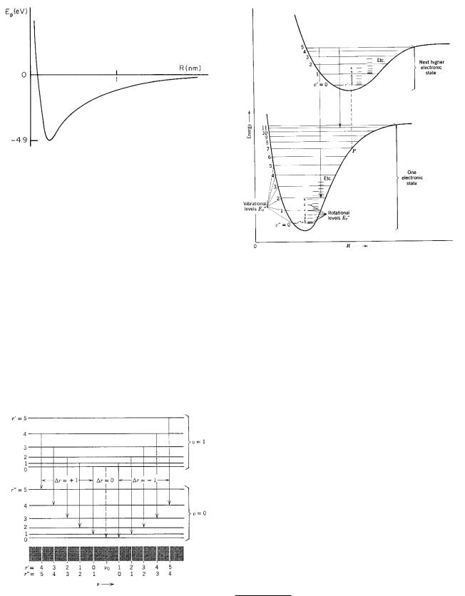
The other possibility is that the atoms in the molecule vibrate back and forth along the line joining their centers. If two masses have an equilibrium position a certain distance apart, work must done either to push them closer together or to pull them farther apart. In either case the potential energy is increased. At the equilibrium separation the potential energy is a minimum. Figure 14.6 shows the potential energy Ep of a sodium ion and a chloride ion as a function of their separation. The potential has a minimum at a separation of about 0.2 nm. The simplest function that has a minimum is a parabola. A parabola can be used to approximate the minimum in Fig. 14.6: Ep(R) = 12 k(R − R0)2. R0 is the equilibrium separation. Since (see Sec. 6.4) dEp = −F dr, the force between the ions is F = −dEp/dR = −k(R − R0), which is the linear approximation to the force between the two ions. The force is attractive if R > R0 and repulsive if R < R0.

A mass subject to a linear restoring force is called a harmonic oscillator (Appendix F). A mass m subject to a linear restoring force −kx oscillates with an angular frequency ω2 = k/m. Classically, the energy of the oscillating mass depends on the amplitude of the motion and can have any value. Quantum-mechanically, it is

364 14. Atoms and Light

FIGURE 14.6. The potential energy of a sodium ion and a chloride ion as a function of their nuclear separation.

This is the total energy, including both kinetic and potential energy. The levels are spaced equally by an amountω. The spacing is usually greater than that for rotational levels, often in the infrared. The transitions that give rise to the emission or absorption of photons require a change in the rotational quantum numbers as well as the vibrational ones. The selection rules are

Some of these vibrational–rotational transitions are shown in Fig. 14.7.

Finally, there can be transitions involving v, r, and the electronic quantum numbers as well. When the electronic quantum numbers change, the shape of the interatomic

FIGURE 14.8. A combination of changes in electronic quantum numbers within an atom and of vibrational and rotational quantum numbers within the molecule. From R. Eisberg and R. Resnick.Quantum Physics of Atoms, Molecules, Solids, Nuclei and Particles, 2nd ed. p. 430. Copyright c 1985 John Wiley & Sons. Reproduced by permission of John Wiley & Sons, Inc.

potential changes, as shown in Fig. 14.8. The details of molecular spectra are fairly involved and are summarized in many texts. Transitions of biological importance are discussed in Grossweiner (1994, pp. 33–38). If the electron selection rules are satisfied, the transition is fairly rapid (typically 10−8 s), a process called fluorescence. Sometimes the electron becomes trapped in a state where it cannot decay according to the electronic selection rules of Eq. 14.9. It may then have a lifetime up to several seconds before decaying, a phenomenon called phosphorescence.

14.4Scattering and Absorption of Radiation; Cross Section

Photons in a vacuum travel in a straight line. When they travel through matter they are apparently3 slowed down, leading to an index of refraction greater than unity; they may also be scattered or absorbed. Visible light does not

FIGURE 14.7. Transitions for vibrational–rotational spectra. From R. M. Eisberg and R. Resnick.Quantum Physics of Atoms, Molecules, Solids, Nuclei and Particles, 2nd ed. p. 428. Copyright c 1985 John Wiley & Sons. Reproduced by permission of John Wiley & Sons, Inc.

3Individual photons travel at speed c, yet the light wave travels at speed c/n. The slowing down of light in a medium is due to interference between the primary beam and scattered photons. This is discussed in Sherwood (1996), in Milonni (1996), and the references cited in these papers.

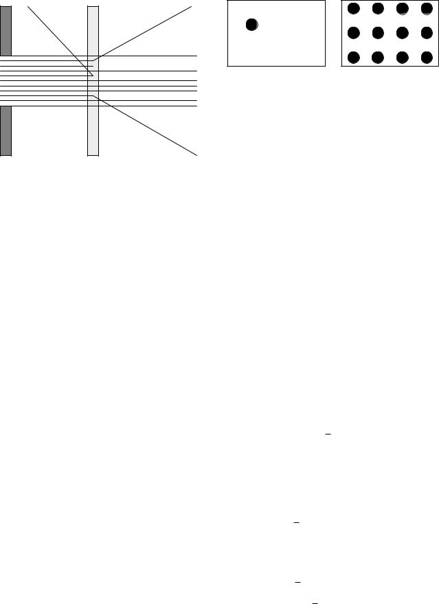
FIGURE 14.9. A collimated beam of photons passes from left to right through a thin slice of material. Some photons pass through, some are scattered, and some are absorbed.

FIGURE 14.10. Each circle represents the cross section σ associated with a target entity such as an atom. (a) There is one atom in area S. (b) There are T target atoms per unit area in area S .

The total number of unscattered photons N changes according to

dN = −(dNs + dNa) = −N (µs + µa)dz

with solution

pass through a building wall, but it does pass through a glass window. The absorption may depend on the frequency or wavelength of the light. The window can be made of colored glass. The light can also be scattered. This leads to the blue of the sky or to the white of clouds. If there is absorption as well as scattering, the clouds may appear gray instead of white. How light is scattered or absorbed in tissue has become very important in biophysics. Infrared light absorption can be used to measure chemical composition of the body. Light is also used for therapy and for laser surgery.

This section shows how to describe a single interaction of a photon with some substance. The photon can be scattered or absorbed. Section 14.5 develops one technique for calculating what happens when the photon undergoes many scattering events before being absorbed or emerging from the material.

Imagine that we have a distant source of photons that travel in straight lines, and that we collimate the beam (send it through an aperture) so that a nearly parallel beam of photons is available to us. Imagine also that we can see the tracks of the N photons in the beam, as in Fig. 14.9. When a thin sample of material of thickness dz is placed in the beam, a certain number of photons are scattered and a certain number are absorbed. If we repeat the experiment many times, we find that the number of photons scattered fluctuates about an average value that we call dNs and the number absorbed fluctuates about an average value dNa. When we vary the thickness of the absorber, we find that if it is su ciently thin, the average number of photons scattered and absorbed is proportional to the thickness as well as the number of incident photons:

The quantity µ is the total linear attenuation coe cient. Quantities µs and µa are the linear scattering and absorption coe cients. Both depend on the material and the energy of the photons. This kind of exponential absorption is known as Beer’s law or the Beer–Lambert law.

The interaction of photons with matter is statistical. The cross section σ is an e ective area proportional to the probability that an interaction takes place. The interaction takes place with a “target entity.” It is sometimes convenient to define the target to be a single molecule, at other times an atom, and still other times one of the electrons within an atom. We can visualize the meaning of the cross section by considering either a single target entity interacting with a beam of photons or a single photon interacting with a thin foil of targets. Both are shown in Fig. 14.10. For the single target in Fig. 14.10(a), consider a beam of N photons passing through the area S with a uniform number per unit area N/S. Let the average number of interactions be n. The cross section per target entity is defined by saying that the fraction of photons that interact is equal to the fraction of the area occupied by the cross section:

We denote the number of photons per unit area by Φ and write Eq. 14.16 as n = σΦ. This is the average number of scatterings per target entity or the probability of interaction per target entity when the beam has Φ photons per unit area:

Strictly speaking, n is dimensionless, σ has the dimensions m2, and Φ has dimensions m−2. However, it is often helpful to think of n as being interactions per target entity and σ as being m2 per target entity.

366 14. Atoms and Light

Alternatively, imagine sending a beam of photons at the target of area S shown in Fig. 14.10(b). There are NT target entities per unit area in the path of the beam, each having an associated area σ. The fraction of the photons that interact is again the fraction of the area that is covered:

This is the probability that a single photon interacts when there are NT target entities per unit area. Note the symmetry with Eq. 14.17. In the first case there is one target entity and a certain number of photons per unit area. In the second case there is one photon and a certain number of target entities per unit area.

If a number of mutually exclusive interactions can take place (such as absorption and scattering), we can define a cross section for each kind of interaction. The probabilities and the cross sections add:

The second interpretation we had above can be used to relate the cross section to the attenuation coe cient. The number of target entities per unit area is equal to the number per unit volume times the thickness of the target along the beam. To obtain the number of target atoms per unit volume, recall that 1 mol of atoms contains Avogadro’s number NA atoms. If A is the mass of a target containing 1 mol of atoms and the target has mass density ρ, then volume V has mass ρV and contains ρV /A mol and NAρV /A atoms. Therefore, the number of atoms per unit volume is NAρ/A, and the number of atoms per unit area is

The linear coe cients are related to their corresponding cross sections by

where σtot is the sum of all the interaction cross sections. Be careful with units! Avogadro’s number is defined to be 6.022137 × 1023 entities per mole, which

is the number in a gram atomic weight. For carbon, A = 12.01 × 10−3 kg mol−1 and ρ = 2.0 × 103 kg m−3.

This is discussed further on p. 409.

We may wish to know the probability that particles (in this case photons) are scattered in a certain direction. We have to consider the probability that they are scattered into a small solid angle dΩ. In this case σ is called the

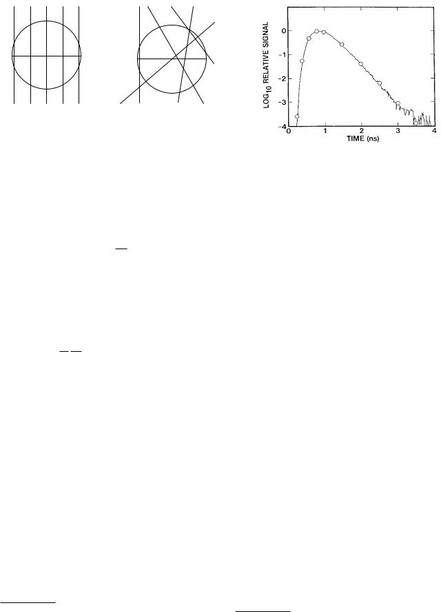
FIGURE 14.11. (a) A small solid angle dΩ = sin θ dθ dφ surrounds the direction defined by angles θ and φ. (b) The solid angle dΩ = 2π sin θ dθ results from integrating over φ.

di erential scattering cross section and is often written as

The units of the di erential scattering cross section are m2 sr−1. The di erential cross section depends on θ, the angle between the directions of travel of the incident and scattered particles. In a spherical coordinate system in which the incident particle moves along the z axis, the solid angle is dΩ = sin θ dθ dφ (Appendix L). If the cross section has no φ dependence, then the integration over φ can be carried out and dΩ = 2π sin θ dθ. These solid angles are shown in Fig. 14.11.

There are three ways to interpret the exponential decay of the beam that has not undergone any interactions. First, the number of particles remaining in the beam that have undergone no interaction decreases as the target becomes thicker, so that the number of particles available to interact in the deeper layers is less. Second, the exponential can be regarded as taking into account the fact that in a thicker sample some of the target atoms are hidden behind others and are therefore less e ective in causing new interactions. The third interpretation is in terms of the Poisson probability distribution (Appendix J). Each layer of thickness dz provides a separate chance for the beam particles to interact. The probability of interacting in any one layer dz is small, p = σtotNAρ dz/A, while the total number of “tries” is z/dz. The average number of interactions is m = p × number of tries. The probability of no interaction is e−m = exp(−σtotNAρ z/A) = e−µz .

When the cross section for scattering is large, things can become quite complicated. For example, photons may scatter many times and be traveling through the material in all directions. Various approximations have been used

to model photon transport in such a case. We will examine some of them shortly. One simple correction that is often made is to consider the average direction a scattered photon travels, for example, the average value of the cosine of the scattering angle, g = cos θ, where θ is the angle of a single scattering. If the average angle of scattering is very small, g is nearly 1. If the photon is scattered backward, g = −1, and if the scattering is isotropic, g = 0. Formally,

The reduced scattering coe cient

is what is usually measured.

The values of the absorption and scattering coe cients vary widely. For infrared light at 780 nm, values are roughly4

14.5The Di usion Approximation to Photon Transport

14.5.1 General Theory

When photons enter a substance, they may scatter many times before being absorbed or emerging from the substance. This leads to turbidity, which we see, for example, in milk or clouds. The most accurate studies of multiple scattering are done with “Monte Carlo” computer simulations, in which probabilistic calculations are used to follow a large number of photons as they repeatedly interact in the tissue being simulated. However, Monte Carlo techniques use lots of computer time. Various approximate analytic solutions also exist. The field is reviewed in Chapter 5 of Grossweiner (1994). One of the approximations, the di usion approximation, is described here. It is valid when many scattering events occur for each photon absorption. This is a valid approximation for most tissue, but not for cerebrospinal fluid or synovial (joint) fluid.

If the photons have undergone enough scattering in a medium, all memory of their original direction is lost. In that case the movement of the photons can be modeled by the di usion equation. In Chapter 4 we wrote Fick’s

second law as

∂C∂t = D 2C + Q.

4These are eyeballed from data for various tissues reported in the article by Yodh and Chance (1995). Values are up to ten times larger at other wavelengths. See Table 5.2 in Grossweiner (1994). Nickell et al. (2000) report values for skin that depend on both the direction of propagation and the degree of stretching of the skin. They are similar to the values reported here.

The left-hand side of the equation is the rate at which the concentration, the number of particles per unit volume, is increasing. The term D 2C is the net di usive flow into the small volume, the particle current being given by j = −D C. The last term is the rate of production or loss of particles within the volume by other processes, depending on whether Q is positive or negative.

Let us suppose that we can apply this to photons. We will consider two contributions to Q. The concentration must be the number of di using photons per unit volume. Any in the incident beam are still traveling in the original direction and are not di using, but if they are scattered they become part of the di using photon pool. Therefore there may be a source term, which we will call s, due to the incident photons. But photons are also being absorbed. They are traveling with a speed cn = c/n, where n is the index of refraction of the medium. In time dt they travel a distance dx = cndt, and the probability that they are absorbed is µadx = µacndt. Therefore, the di usion equation for photons is

Each term has the units of photons m−3 s−1.

In photon transfer, it is customary to make two changes in this equation. The first is to divide all terms by the speed of the photons in the medium,5 cn. The result is

where D = D/cn is referred to in the photon transfer literature as the photon di usion constant. It has dimensions of length.

Two important quantities in radiation transfer are the photon or particle fluence and the photon fluence rate. The International Commission on Radiation Units and Measurements (ICRU) defines the particle fluence for any kind of particle, including photons as follows: At the point of interest construct a small sphere of radius a. Let the number of particles striking the surface of the sphere during some time interval have an expectation value N . (The expectation value is the mean of a set of measurements in the limit as the number of measurements becomes infinite.)

The particle fluence Φ is the ratio N/πa2, where πa2 is the area of a great circle of the sphere, that is, the area of a circle having the same radius as the sphere. This is shown in Fig. 14.12 and is a generalization of our earlier use of Φ as the number of particles per unit area. It neatly avoids having to introduce obliquity factors, since for any direction the particles travel, one can construct a great circle on the sphere that is perpendicular to their path.

5Most papers in this field use c as the velocity of light in the medium. We prefer to reserve c for the fundamental constant, the velocity of light in vacuum.

FIGURE 14.12. The particle fluence is the ratio of the expectation or average value of the number of particles passing through the sphere to the area of a great circle of the sphere, πa2. It depends on the total number of particles passing through the sphere, regardless of the direction they travel. The fluence is the same in each case shown: five particles traverse each sphere.

The particle fluence rate is

ϕ = ddtΦ .

FIGURE 14.13. Time-resolved infrared spectroscopy. The line is a measurement of the reflected photons from the calf of a human volunteer at a distance of 4 cm from the pulsed source. The wavelength is 760 nm. The circles are calculated using Eq. 14.29 and normalized to the peak value. From M. S. Patterson, B. Chance, and B. C. Wilson (1989). Time resolved reflectance and transmittance for the noninvasive measurement of tissue optical properties. Appl. Opt. 28(12): 2331–2336. Copyright by the Optical Society of America.

We saw in Chapter 4 that for a group of particles all traveling with the same speed, the number transported across a plane per unit area per unit time is equal to their concentration times their speed. The photon concentration is related to the photon fluence rate by C = ϕ/cn, and the photon di usion equation becomes

This is the form that is usually found in the literature. The units of each term are photons m−3 s−1. One can show that6

14.5.2 Continuous Measurements

If the tissue is continuously irradiated with photons at a constant rate, the term containing the time derivative vanishes. If in addition we use a broad beam of photons so that we have a one-dimensional problem and we are far enough into the tissue so that the source term can be ignored, the model is

This has an exponential solution ϕ = ϕ0e−µeffx, where µe = {3µa [µa + (1 − g)µs]}1/2. It is interesting to see

6See, for example, Duderstadt and Hamilton (1976, pp. 133– 136).

what these numbers mean. Using the “typical” values from Sec. 14.4, the number of photons that have not interacted (are not yet attenuated) falls exponentially with a characteristic length or mean depth

For the di use beam the mean depth is about 10 times this:

These values are for a wavelength where the tissue is fairly transparent. The di usion equation can be solved for other geometries that model the light source being used.7 One problem with these measurements is that they give only µe , which is a combination of µa and µs. Also, the path length may be ambiguous because the geometry cannot be modeled accurately.

14.5.3 Pulsed Measurements

A technique made possible by ultrashort light pulses from a laser is time-dependent di usion. It allows determination of both µs and µa. A very short (150-ps) pulse of light strikes a small region on the surface of the tissue. A detector placed on the surface about 4 cm away records the multiply-scattered photons. A typical plot of the detected photon fluence rate is shown in Fig. 14.13.

7See, for example, Grossweiner (1994, p. 98).

Patterson et al. (1989) have shown that the reflected fluence rate after a pulse is approximately

Here r is the distance of the detector from the source along the surface of the skin, cnt is the total distance the photon has traveled before detection, and z0 = 1/ [(1 − g)µs] is the depth at which all the incident photons are assumed to scatter and become part of the diffuse photon pool. This curve fits Fig. 14.13 well and can be used to determine µa and (1 − g)µs. We can understand the various factors in Eq. 14.29. The last factor is a Gaussian spreading in the r direction away from the z axis where the photons were injected. This is a two-dimensional problem. Compare this with Eq. 4.77, which shows that in two dimensions σr2 = 4Dt, and recall that D = D cn. The middle factor is the fraction of the photons in the pulse that have not been absorbed, exp(−µax), where x is the total distance the photons have traveled. The first factor is the normalization that reduces the amplitude of the Gaussian as it spreads.

A related technique is to apply a continuous laser beam, the amplitude for which is modulated at various frequencies between 50 and 800 MHz. The Fourier transform of Eq. 14.29 gives the change in amplitude and phase of the detected signal. Their variation with frequency can also be used to determine µa and µs.8

14.5.4 Refinements to the Model

The di usion equation, Eq. 14.26, is an approximation, and the solution given, Eq. 14.29, requires some unrealistic assumptions about the boundary conditions at the surface of the medium (z = 0). Hielscher et al. (1995) compared experiment, Monte Carlo calculations, and solutions to the di usion equation with three di erent boundary conditions. They found that Eq. 14.29 was the easiest to use but leads to errors in the estimates of the coe cients that become worse when the detector and source are close together. Their Monte Carlo calculations fit the data quite well. They also discuss the reflections that occur when light goes from one medium into another with a di erent index of refraction.

14.6Biological Applications of Infrared Scattering

14.6.1 Near Infrared (NIR)

Near infrared light in the range 600–1000 nm is used to measure the oxygenation of the blood as a function of

8See, for example, Sevick et al. (1991) or Pogue and Patterson (1994).

FIGURE 14.14. The absorption coe cient µa for water, oxyhemoglobin, and deoxyhemoglobin. Reprinted with permission from A. Yodh and B. Chance. Spectroscopy and imaging with di using light. Phys. Today, March 1995: 34–40 Copyright c 1995, American Institute of Physics.

time by determining the absorption at two di erent wavelengths. Figure 14.14 shows the absorption coe cients for oxygenated and deoxygenated hemoglobin and water. The greater absorption of blue light in oxygenated hemoglobin makes oxygenated blood red. (The graph only shows wavelengths longer than 600 nm—red and infrared.) The wavelength 800 nm at which both forms of hemoglobin have the same absorption is called the isosbestic point. Measurements of oxygenation are made by comparing the absorption at two wavelengths on either side of this point.

One of the di culties with these measurements is knowing the path length, since photons undergo many scatterings before being absorbed or reaching the detector. Scattering from many tissues besides hemoglobin distorts the signal. Nonetheless, pulse oximeters that fit over a finger are widely used. Webster (1997) provides a comprehensive discussion of the underlying physics, design, calibration and use of pulse oximeters. The basic feature is that arterial blood flow is pulsatile, not continuous. Therefore, measuring the time-varying (AC) signal selectively monitors arterial blood and eliminates the contribution from venous blood and tissue. Scattering corrections must still be made [Farmer (1997), Wieben (1997)].

Development of new applications for infrared scattering measurements continue as new detectors with di erent spectral sensitivities become available [Yamashita et al. (2001)]. Continuous sources are also used to determine blood oxygenation of tissue [Liu et al. (1995)].