Intermediate Physics for Medicine and Biology - Russell K. Hobbie & Bradley J. Roth
.pdf
|
|
|
|
|
|
|
Problems |
431 |
|||
Symbol |
Use |
Units |
First |
|
|
Stopping cross section |
J m2 |
|
415 |
||
|
|
|
used on 0 |
Electrical permittivity |
N−1 C2 m−2 |
|
406 |
||||
|
|
|
page |
|
|
of empty space |
|
|
|
|
|
Ai, Amol |
Atomic mass number |
(g mol)−1 or |
410 |
θ, φ |
Angles |
m2 |
|
405 |
|||
|
of constituent i or |
(kg mol)−1 |
|
κ |
Pair production cross |
|
403 |
||||
|
molecule |
|
|
|
|
section |
|
|
|
|
|
AK |
Auger yield |
|
411 |
λ |
Wavelength |
m |
|
405 |
|||
B, BK , etc. |
Binding energy |
eV or J |
403 |
µ, µatten |
Attenuation coe cient |
m−1 |
|
408 |
|||
B |
Buildup factor or |
|
430 |
µen |
Energy absorption |
m−1 |
|
413 |
|||
|
backscatter factor |
|
|
|
|
coe cient |
m−1 |
|
|
||
C |
Shell correction |
|
420 |
µtr |
Energy transfer |
|
413 |
||||
|
coe cient |
|
|
|
|
coe cient |
|
|
|
|
|
D |
Absorbed dose |
J kg−1 or Gy |
427 |
ν |
Frequency |
Hz |
|
403 |
|||
|
|
(gray) |
|
ξ |
Position |
m |
|
419 |
|||
E |
Energy |
J |
403 |
ρ |
Density |
kg m−3 |
|
408 |
|||
E |
Electric field |
V m−1 |
406 |
σC |
Total Compton cross |
m2 |
|
403 |
|||
F |
Force |
N |
416 |
|
|
section for one electron |
m2 |
|
|
||
F |
Fraction of charged |
|
423 |
σcoh |
Coherent Compton |
|
403 |
||||
|
particles passing |
|
|
|
|
cross section for one |
|
|
|
|
|
|
through an absorber |
|
|
|
|
atom |
m2 |
|
|
||
I |
Average ionization |
eV or J |
420 |
σincoh |
Incoherent Compton |
|
403 |
||||
|
energy |
|
|
|
|
cross section for one |
|
|
|
|
|
I |
Stopping interaction |
J m2 |
420 |
|
|
atom |
m2 |
|
|
||
|
strength |
|
|
σtr |
Transfer cross section |
|
407 |
||||
K, KC |
Kerma, collision kerma |
J |
427 |
σtot |
Total cross section |
m2 |
|
409 |
|||
L |
Stopping number per |
|
420 |
τ |
Photoelectric cross sec- |
m2 |
|
404 |
|||
|
atomic electron |
|
|
|
|
tion |
|
|
|
|
|
L∆ |
Restricted linear |
J m−1 |
423 |
∆ |
Energy transfer |
J |
|
423 |
|||
|
stopping power |
|
|
Φ |
Particle fluence |
m−2 |
|
412 |
|||
M |
Mass |
kg |
410 |
Ψ |
Energy fluence |
J m−2 |
|
412 |
|||
N |
Number of particles |
|
408 |
Ω |
Solid angle |
sr |
|
406 |
|||
NA |
Avogadro’s number |
mol−1 |
408 |
|
|
|
|
|
|
|
|
NT |
Number of target |
m−2 |
410 |
Problems |
|
|
|
|
|
||
|
atoms per unit |
|
|
|
|
|
|
|
|
|
|
|
projected area |
|
|
Section 15.1 |
|
|
|
|
|||
NT V |
Number of target |
m−3 |
410 |
|
|
|
|
||||
|
atoms per unit volume |
|
|
Problem 1 The quantum numbers ms = ±21 and ml = |
|||||||
Q |
Energy released from |
J |
427 |
||||||||
|
rest mass |
|
|
l, l−1, l−2 . . . , −l are sometimes used instead of j and mj |
|||||||
R |
Range |
m |
423 |
to describe an electron energy level. Show that the total |
|||||||
Ru, Rc |
Radiant energy in the |
J |
427 |
number of states for given values of n and l is the same |
|||||||
|
form of uncharged or |
|
|
when either set is used. |
|
|
|
|
|||
|
charged particles |
|
|
|
|
|
|
||||
|
|
|
|
|
|
|
|
|
|
||
S |
Area |
m2 |
427 |
Problem 2 Use Eq. 15.3 to estimate the K-shell ener- |
|||||||
S |
Stopping power |
J m−1 |
415 |
||||||||
gies for the following elements and compare them to the |
|||||||||||
Se |
Electron (collision) |
J m−1 |
416 |
||||||||
|
stopping power |
J m−1 |
|
measured values of EK . |
|
|
|
|
|||
Sn |
Nuclear stopping power |
416 |
|
Z |
Element Measured EK (keV) |
|
|
||||
Sr |
Radiative stopping |
J m−1 |
416 |
|
|
|
|||||
|
power |
|
|
|
|
|
|
|
|
|
|
|
|
|
6 |
Carbon |
0.284 |
|
|
|
|||
T |
Kinetic energy |
J |
403 |
|
|
|
|||||
20 |
Calcium |
4.04 |
|
|
|
||||||
V |
Volume |
m3 |
410 |
|
|
|
|||||
V |
Velocity |
m s−1 |
419 |
53 |
Iodine |
33.2 |
|
|
|
||
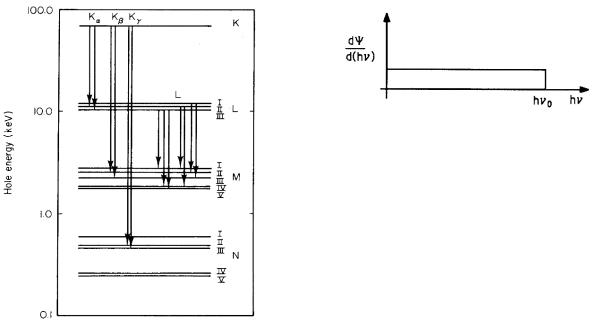
WK,L,M |
Probability that a hole |
|
411 |
82 |
Lead |
88.0 |
|
|
|
||
|
in the K, L, or M shell |
|
|
|
|
|
|
|
|
|
|
|
is filled by fluorescence |
|
|
|
|
|
|
|
|
|
|
W |
Energy lost in a single |
J |
415 |
Section 15.3 |
|
|
|
|
|||
|
interaction |
|
|
Problem 3 The K-shell photoelectric cross section for |
|||||||
Y |
Radiation yield |
|
424 |
||||||||
Z |
Atomic number of |
|
402 |
100-keV photons on lead (Z = 82) is τ = 1.76 |
× |
10−25 |
|||||
|
target atom |
|
|
|
|
|
|
|
|
||
β |
v/c |
|
415 |
m2 atom−1. Estimate the photoelectric cross section for |
|||||||
|
60-keV photons on calcium (Z = 20). |
|
|
||||||||
δ |
Average energy |
J |
413 |
|
|
||||||
|
|
|
|
|
|
|
|||||
|
emitted as fluorescence |
|
|
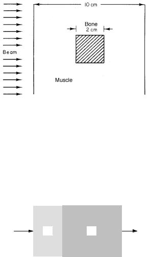
Problem 4 Describe how you could use di erent mate- |
|||||||
|
radiation per photon |
|
|
||||||||
|
|
|
rials to determine the energy of monoenergetic x rays of |
||||||||
|
absorbed |
|
|
||||||||
δ |
Density-e ect |
|
420 |
energy about 50 keV by using changes in the attenuation |
|||||||
|
correction |
|
|
coe cient. What materials would you use? |
|
|
|||||


 e
e hν
hν
|
|
|
|
|
References |
435 |
Hubbell, J. H., P. N. Trehan, N. Singh, B. Chand, D. |
Kissel, L. H., R. H. Pratt, and S. C. Roy (1980). |
|||||
Mehta, M. L. Garg, R. R. Garg, S. Singh, and S. Puri |
Rayleigh scattering by neutral atoms, 100 eV to 10 MeV. |
|||||
(1994). A review, bibliography, and tabulation of K, L, |
Phys. Rev. A. 22: 1970–2004. |
|
||||
and higher atomic shell x-ray fluorescence yields. J. Phys. |
Powell, C. F., P. H. Fowler, and D. H. Perkins (1959). |
|||||
Chem. Ref. Data 23(2): 339–364. |
|
|
|
The Study of Elementary Particles by the Photographic |
||
ICRU Report 16 (1970). Linear Energy Transfer. |
Method. New York, Pergamon. |
|
||||
Bethesda, MD, International Commission on Radiation |
Pratt, R. H. (1982). Theories of coherent scattering of |
|||||
Units and Measurements. |
|
|
|
x rays and γ rays by atoms, in Proceedings of the Second |
||
ICRU Report 33 (1980). Radiation Quantities and |
Annual Conference of International Society of Radiation |
|||||
Units. Bethesda, MD, International Commission on Ra- |
Physicists, Penang, Malaysia. |
|
||||
diation Units and Measurements. |
|
|
|
Rossi, B. (1957). Optics. Reading, MA, Addison- |
||
ICRU Report 37 (1984). Stopping Powers for |
Wesley, Chapter 8. |
|
||||
Electrons and Positrons. Bethesda, MD, Inter- |
Seltzer, S. M. (1993). Calculation of photon mass |
|||||
national Commission on Radiation Units and |
energy-transfer and mass energy-absorption coe cients. |
|||||
Measurements. |
Information |
also |
available |
at |
Radiat. Res. 136: 147–170. |
|
physics.nist.gov/PhysRefData/Star/Text/contents.html. |
Tung, C. J., J. C. Ashley, and R. H. Ritchie (1979). |
|||||
ICRU Report 49 (1993). Stopping Powers and |
Range of low-energy electrons in solids. IEEE Trans. |
|||||
Ranges for Protons and Alpha Particles. Bethesda, |
Nucl. Sci. NS-26: 4874–4878. |
|
||||
MD, International Commission |
on |
Radiation |
Units |
Ziegler, J. F., and J. M. Manoyan (1988). The stopping |
||
and Measurements. Information also available at |
of ions in compounds. Nucl. Instrum. Methods in Phys. |
|||||
physics.nist.gov/PhysRefData/Star/Text/contents.html. |
Res. B35: 215–228. |
|
||||
Jackson, D. F., and D. J. Hawkes (1981). X-ray attenu- |
Ziegler, J. F., J. P. Biersack, and U. Littmark (1985). |
|||||
ation coe cients of elements and mixtures. Phys. Reports |
The Stopping and Range of Ions in Solids. New York, |
|||||
70: 169–233. |
|
|
|
|
Pergamon. |
|