Intermediate Physics for Medicine and Biology - Russell K. Hobbie & Bradley J. Roth

A.1 Plane Angles

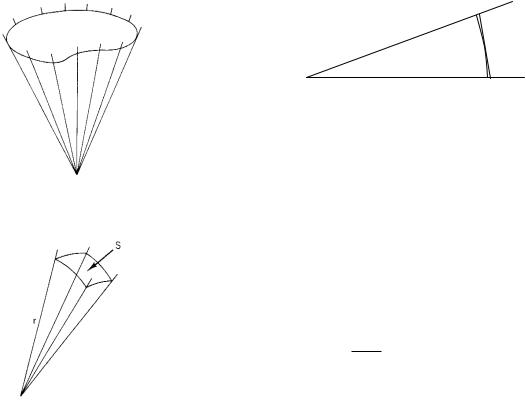
The angle θ between two intersecting lines is shown in Fig. A.1. It is measured by drawing a circle centered on the vertex or point of intersection. The arc length s on that part of the circle contained between the lines measures the angle. In daily work, the arc length is marked o in degrees.

In some cases, there are advantages to measuring the angle in radians. This is particularly true when trigonometric functions have to be di erentiated or integrated. The angle in radians is defined by

Since the circumference of a circle is 2πr, the angle corresponding to a complete rotation of 360 ◦ is 2πr/r = 2π. Other equivalences are

10.01745

Since the angle in radians is the ratio of two distances, it is dimensionless. Nevertheless, it is sometimes useful to

θ (degrees)

FIGURE A.2. Comparison of y = tan θ, y = θ (radians), and y = sin θ.

specify that something is measured in radians to avoid confusion.

One of the advantages of radian measure can be seen in Fig. A.2. The functions sin θ, tan θ, and θ in radians are plotted vs angle for angles less than 80 ◦. For angles less than 15 ◦, y = θ is a good approximation to both

y = tan θ (2.3% error at 15 ◦) and y = sin θ (1.2% error at 15 ◦).

A.2 Solid Angles

FIGURE A.1. A plane angle θ is measured by the arc length s on a circle of radius r centered at the vertex of the lines defining the angle.

A plane angle measures the diverging of two lines in two dimensions. Solid angles measure the diverging of a cone of lines in three dimensions. Figure A.3 shows a series of

544 Appendix A. Plane and Solid Angles

FIGURE A.3. A cone of rays in three dimensions.

FIGURE A.4. The solid angle of this cone is Ω = S/r2. S is the surface area on a sphere of radius r centered at the vertex.

rays diverging from a point and forming a cone. The solid angle Ω is measured by constructing a sphere of radius r centered at the vertex and taking the ratio of the surface area S on the sphere enclosed by the cone to r2:

This is shown in Fig. A.4 for a cone consisting of the planes defined by adjacent pairs of the four rays shown. The unit of solid angle is the steradian (sr). A complete

FIGURE A.5. For small angles, the arc length is very nearly equal to the length of the tangent to the circle.

sphere subtends a solid angle of 4π steradians, since the surface area of a sphere is 4πr2.

When the included angle in the cone is small, the difference between the surface area of a plane tangent to the sphere and the sphere itself is small. (This is di - cult to draw in three dimensions. Imagine that Fig. A.5 represents a slice through a cone; the di erence in length between the circular arc and the tangent to it is small.) This approximation is often useful. A 3 × 5-in. card at a distance of 6 ft (72 in.) subtends a solid angle which is approximately

3 × 5 = 2.9 × 10−3 sr. 722

It is not necessary to calculate the surface area on a sphere of 72 in. radius.

Problems

Problem 1 Convert 0.1 radians to degrees. Convert 7.5 ◦ to radians.

Problem 2 Use the fact that sin θ ≈ θ ≈ tan θ to estimate the sine and tangent of 3 ◦. Look up the values in a table and see how accurate the approximation is.

Problem 3 What is the solid angle subtended by the pupil of the eye (radius = 3 mm) at a source of light 30 m away?

B.1 Vectors and Vector Addition

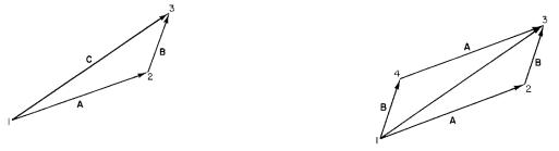
A displacement describes how to get from one point to another. A displacement has a magnitude (how far point 2 is from point 1 in Fig. B.1) and a direction (the direction one has to go from point 1 to get to point 2). The displacement of point 2 from point 1 is labeled A. Displacements can be added: displacement B from point 2 puts an object at point 3. The displacement from point 1 to point 3 is C and is the sum of displacements A and

B:

A displacement is a special example of a more general quantity called a vector. One often finds a vector defined as a quantity having a magnitude and a direction. However, the complete definition of a vector also includes the requirement that vectors add like displacements. The rule for adding two vectors is to place the tail of the second vector at the head of the first; the sum is the vector from the tail of the first to the head of the second.

A displacement is a change of position so far in such a direction. It is independent of the starting point. To know where an object is, it is necessary to specify the starting point as well as its displacement from that point.

Displacements can be added in any order. In Fig. B.2, either of the vectors A represents the same displacement. Displacement B can first be made from point 1 to point 4, followed by displacement A from 4 to 3. The sum is still C:

The sum of several vectors can be obtained by first adding two of them, then adding the third to that sum, and so forth. This is equivalent to placing the tail of each vector at the head of the previous one, as shown in Fig. B.3. The sum then goes from the tail of the first vector to the head of the last.

The negative of vector A is that vector which, added to A, yields zero:

It has the same magnitude as A and points in the opposite direction.

Multiplying a vector A by a scalar (a number with no associated direction) multiplies the magnitude of vector A by that number and leaves its direction unchanged.

4

2

1

FIGURE B.3. Addition of several vectors.

FIGURE B.4. Vector A has components Ax and Ay .

B.2 Components of Vectors

Consider a vector in a plane. If we set up two perpendicular axes, we can regard vector A as being the sum of vectors parallel to each of these axes. These vectors, Ax and Ay in Fig. B.4, are called the components of A along each axis1. If vector A makes an angle θ with the x axis and its magnitude is A, then the magnitudes of the components are

The sum of the squares of the components is A2x + A2y = A2 cos2 θ + A2 sin2 θ = A2(sin2 θ + cos2 θ). Since, by Pythagoras’ theorem, this must be A2, we obtain the trigonometric identity

In three dimensions, A = Ax + Ay + Az . The magnitudes can again be related using Pythagoras’ theorem, as

shown in Fig. B.5. From triangle OP Q, A2xy = A2x + A2y . From triangle OQR,

In our notation, Ax means a vector pointing in the x direction, while Ax is the magnitude of that vector. It can

1Some texts define the component to be a scalar, the magnitude of the component defined here.

FIGURE B.5. Addition of components in three dimensions.

become di cult to keep the distinction straight. Therefore, it is customary to write xˆ, yˆ, and ˆz to mean vectors of unit length pointing in the x, y, and z directions. (In

ˆ

some books, the unit vectors are denoted by ˆı, ˆ, and k instead of xˆ, yˆ, and ˆz.) With this notation, instead of Ax, one would always write Axxˆ.

The addition of vectors is often made easier by using components. The sum A + B = C can be written as

Axxˆ + Ay yˆ + Azˆz + Bxxˆ + By yˆ + Bzˆz

= Cxxˆ + Cy yˆ + Czˆz.

Like components can be grouped to give

(Ax + Bx)xˆ + (Ay + By )yˆ + (Az + Bz )ˆz

= Cxxˆ + Cy yˆ + Czˆz.

Therefore, the magnitudes of the components can be added separately:

B.3 Position, Velocity, and

Acceleration

The position of an object at time t is defined by specifying its displacement from an agreed-upon origin:

R(t) = x(t)xˆ + y(t)yˆ + z(t)ˆz.

The average velocity vav(t1, t2) between times t1 and t2 is defined to be

vav(t1, t2) = R(t2) − R(t1) .

t2 − t1

This can be written in terms of the components as

The x component of the velocity tells how rapidly the x component of the position is changing.

The acceleration is the rate of change of the velocity with time. The instantaneous acceleration is

Problems 547

a(t) = ddtv = dvdtx xˆ + dvdty yˆ + dvdtz ˆz.

Problems

Problem 1 At t = 0, the position of an object is given by R = 10xˆ + 5yˆ, where R is in meters. At t = 3 s, the position is R = 16xˆ−10yˆ. What was the average velocity between t = 0 and 3 s?

In the expression am, a is called the base and m is called the exponent. Since a2 = a ×a, a3 = a ×a ×a, and

The most useful property of logarithms can be derived by letting

am = (a × a × a × · · · × a),

m times

it is easy to show that

aman = (a × a × a × · · · × a)(a × a × a × · · · × a),

If m > n, the same technique can be used to show that

If m = n, this gives

1 = am = am−m = a0, am

The rules also work for m < n and for negative exponents. For example,

If y = ax, then by definition, x is the logarithm of y to the base a: x = loga(y). If the base is 10, since 100 = 102, 2 = log10(100). Similarly, 3 = log10(1000), 4 = log10(10000), and so forth.

All logarithms in this book, unless labeled with a specific base, are to base e (see Chap. 2). These are the so-called natural logarithms. We will denote the natural logarithm by ln, using log10 when we want logarithms to the base 10.

Problems

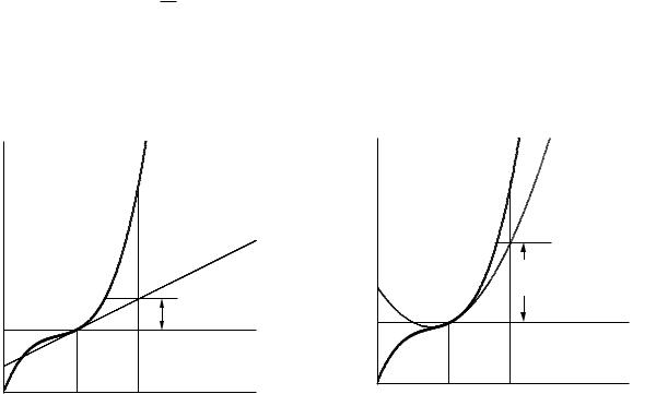
Consider the function y(x) shown in Fig. D.1. The value of the function at x1, y1 = y(x1), is known. We wish to estimate y(x1 + ∆x).

The simplest estimate, labeled approximation 0 in Fig. D.1, is to assume that y does not change: y(x1 + ∆x) ≈ y(x1). A better estimate can be obtained if we assume that y changes everywhere at the same rate it does at x1. Approximation 1 is

dy

y(x1 + ∆x) ≈ y(x1) + ∆x. dx x1

The derivative is evaluated at point x1.

An even better estimate is shown in Fig. D.2. Instead of fitting the curve by the straight line that has the proper first derivative at x1, we fit it by a parabola that matches both the first and second derivatives. The approximation

is

That this is the best approximation can be derived in the following way. Suppose the desired approximation is more general and uses terms up to (∆x)n = (x − x1)n:

yapprox = A0 +A1(x−x1)+A2(x−x1)2 +· · ·+An(x−x1)n

(D.1)

The constants A0, A1, . . . , An are determined by making the value of yapprox and its first n derivatives agree with the value of y and its first n derivatives at x = x1. When x = x1, all terms with x − x1 in yapprox vanish, so that

yapprox(x1) = A0.

y(x)

y

Approximation 2

(dy/dx)|x1∆x

+ (1/2)(d2y/dx2)|x1(∆x)2

Evaluating these at x = x1 gives

d2(yapprox)

dx2 = 2 × 1 × A2,

x1

d3(yapprox)

dx3 = 3 × 2 × 1 × A3,

x1

dn(yapprox)

dxn = n!An.

x1

FIGURE D.4. An enlargement of Fig. D.3 near x = 0.

Combining these expressions for An with Eq. D.1, we get

Tables D.1 and D.2 and Figs. D.3 and D.4 show how the Taylor’s series approximation gets better over a larger and larger region about x1 as more terms are added. The function being approximated is y = e2x. The derivatives

are given in Table D.1. The expansion is made about x1 = 0.

Finally, the Taylor’s series expansion for y = ex about x = 0 is often useful. Since all derivatives of ex are ex, the value of y and each derivative at x = 0 is 1. The series is

(Note that 0! = 1 by definition.)

Problems 553

Problems

Problem 1 Make a Taylor’s series expansion of y = a + bx + cx2 about x = 0. Show that the expansion exactly reproduces the function.

Problem 2 Repeat the previous problem, making the expansion about x = 1.

d(sin x)/dx = cos x and d(cos x)/dx = − sin x.

(b) Make a Taylor’s series expansion of the sine function.

The average of a function of x with period T is defined to be

The sine function is plotted in Fig. E.1(a). The integral over a period is zero, and its average value is zero. The area above the axis is equal to the area below the axis. Figure E.1(b) shows a plot of sin2 x. Since sin x varies between −1 and +1, sin2 x varies between 0 (when sin x = 0) and +1 (when sin x = ±1). Its average value, from inspection of Fig. E.1(b) is 12 . If you do not want to trust the drawing to convince yourself of this, recall the identity sin2 θ + cos2 θ = 1. Since the sine function and the cosine function look the same, but are just shifted along the axis, their squares must also look similar. Therefore, sin2 θ and cos2 θ must have the same average. But if their sum is always 1, the sum of their averages must be 1. If the two averages are the same, then each must be 12 .

These same results could have been obtained analyti-

The integrals of sin x and cos x are

These could be used to show that the average value of sin x or cos x is zero. Then Eq. E.2 could be used to show that the average of sin2 x is 12 .

The integral of sin2 x over a period is its average value times the length of the period:

We will also encounter integrals like

T

sin mx sin nx dx, m =n,

0

All these integrals are zero. This can be shown using integral tables. Or, you can see why the integrals vanish by considering the specific examples plotted in Fig. E.2. Each integrand has equal positive and negative contributions to the total integral.