

Intermediate Physics for Medicine and Biology - Russell K. Hobbie & Bradley J. Roth
.pdf568 Appendix I. The Gaussian Probability Distribution
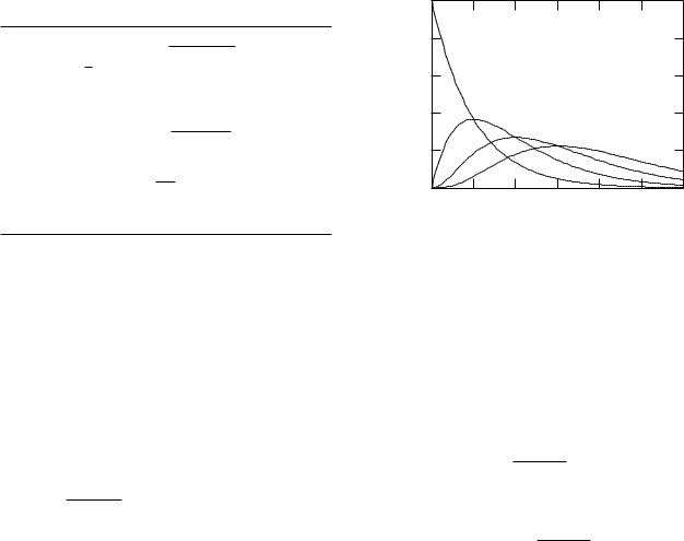
TABLE I.1. Accuracy of Stirling’s approximation.
n |
n! |
|
ln(n!) |
n ln n − n |
Error |
% Error |
5 |
120 |
4.7875 |
3.047 |
1.74 |
36 |
|
|
|
6 |
15.104 |
13.026 |
2.08 |
14 |
10 |
3.6 |
× 1018 |
||||
20 |
2.4 |
× 10157 |
42.336 |
39.915 |
2.42 |
6 |
100 |
9.3 |
× 10 |
363.74 |
360.51 |
3.23 |
0.8 |
FIGURE I.2. Evaluating the normalization constant.
We can now return to the task of deriving the binomial distribution. Taking logarithms of Eq. I.1, we get
y= ln P = ln(N !) − ln(n!) − ln(N − n)!
+n ln p + (N − n) ln(1 − p).
With Stirling’s approximation, this becomes
y= N ln N − n ln n − N ln(N − n) + n ln(N − n)
|
|
+ n ln p + (N − n) ln(1 − p). |
(I.3) |
|||||||
The derivative with respect to n is |
|
|||||||||
|
dy |
= − ln n + ln(N |
− n) + ln p − ln(1 |
− p). |
||||||
|
|
|||||||||
dn |
||||||||||
The second derivative is |
|
|
|
|
|
|
||||
|
|
|
d2y |
1 |
1 |
|
|
|||
|
|
|
|
= − |
|
− |
|
. |
|
|
|
|
|
dn2 |
n |
N − n |
|
||||
The point of expansion n0 is found by making the first derivative vanish:
0 = ln (N − n)p . n(1 − p)
Since ln 1 = 0, this is equivalent to (N −n0)p = n0(1 −p) or n0 = N p. The maximum of y occurs when n is equal to the mean. At n = n0 the value of the second derivative
is |
1 |
1 |
1 |
|
||||
|
d2y |
|
||||||
|
|
= − |
|
− |
|
= − |
|
. |
dn2 |
N p |
N (1 − p) |
N p(1 − p) |
|||||
It is still necessary to evaluate y0 = y(n0). If we try to do this by substitution of n = n0 in Eq. I.3, we get zero. The reason is that the Stirling approximation we used is too crude for this purpose. (There are additional terms in Stirling’s approximation that make it more accurate.) The easiest way to find y(n0) is to call it y0 for now and determine it from the requirement that the probability be normalized. Therefore, we have
y = y0 − 1 (n − N p)2
2N p(1 − p) so that, in this approximation,
P (n) = ey = ey0 e−(n−N p)2/[2N p(1−p)].
With N p = n, ey0
P (n) = C0e−(n−n)2/2σ2 .
FIGURE I.3. The allowed values of x are closely spaced in this case.
To evaluate C0, note that the sum of P (n) for all n is the area of all the rectangles in Fig. I.2. This area is approximately the area under the smooth curve, so that
∞
1 = C0 |
e−(n− |
|
)2/2σ2 |
|
n |
dn. |
|||
|
−∞ |
|
||
It is shown in Appendix K that half of this integral is
∞ |
bx2 |
1 |
" |
π |
||
dx e− |
= |
|
|
|
|
. |
2 |
|
|||||
0 |
|
|
b |
|||
Therefore the normalization integral is (letting x = n−n)
∞ e−x2/2σ2 dx = √2πσ2.
−∞
√
The normalization constant is C0 = 1/ 2πσ2, so that the Gaussian or normal probability distribution is
P (n) = √ 1 . (I.4) 2πσ2
It is possible, as in the case of the random-walk problem, that the measured quantity x is proportional to n with a very small proportionality constant, x = kn, so that the values of x appear to form a continuum. As shown in Fig. I.3, the number of di erent values of n [each with about the same value of P (n)] in the interval dx is proportional to dx. The easiest way to write down the Gaussian distribution in the continuous case is to recognize that the mean is x = kn, and the standard deviation
is σx2 = (x − x)2 = x2 − x2 = k2n2 − k2n2 = k2σ2. The term P (x)dx is given by P (n) times the number
of di erent values of n in dx. This number is dx/k.

Therefore, |
|
|
|
|
|
|
|
|
|
|
|
|
|
|
|
|
|
|
|
dx |
1 |
|
|
2 |
|
2 |
|||||||
P (x)dx = P (n) |
|
|
= dx |
k√ |
|
e−(x/k−x/k) |
/2σ |
|
||||||||
k |
|
|
||||||||||||||
2πσ2 |
|
|
||||||||||||||
= dx |
|
|
1 |
|
|
|
2 |
2 |
|
|
|
(I.5) |
||||
|
|
|
|
|
e−(x−x) |
/2σx . |
|
|||||||||
|
|
|
|
|
|
|||||||||||
|
√2πσx |
|
|
|
|
|
|
|||||||||
Appendix I. The Gaussian Probability Distribution |
569 |
To recapitulate: the binomial distribution in the case of large N can be approximated by Eq. I.4, the Gaussian or normal distribution, or Eq. I.5 for continuous variables. The original parameters N and p are replaced in these approximations by n (or x) and σ.

Appendix J
The Poisson Distribution
Appendix H discussed the binomial probability distribution. If an experiment is repeated N times, and has two possible outcomes, with “success” occurring with probability p in each try, the probability of getting that outcome x times in N tries is
P (x; N, p) = |
N ! |
|
px(1 − p)N −x. |
|
x!(N |
− |
x)! |
||
|
|
|
|
|
The distribution of possible values of x is characterized by a mean value x = N p and a variance σ2 = N p(1 − p). It is possible to specify x and σ2 instead of N and p to define the distribution.
Appendix I showed that it is easier to work with the Gaussian or normal distribution when N is large. It is specified in terms of the parameters x and σ2 instead of N and p:
P (x; |
x, σ2) = |
1 |
|
|
2 |
2 |
|
||||||
|
e−(x−x) |
/2σ . |
||||
(2πσ2)1/2 |
||||||
The Poisson distribution is an approximation to the binomial distribution that is valid for large N and for small p (when N gets large and p gets small in such a way that their product remains finite). To derive it, rewrite the binomial probability in terms of p = x/N :
P (x) = |
N ! |
|
( |
x/N )x(1 − |
x/N )N −x |
|
||||||||||||||
|
|
|
|
|||||||||||||||||
x!(N |
− |
x)! |
|
|||||||||||||||||
|
|
1 |
|
|
|
|
|
|
|
|
N |
|
|
|
|
−x |
||||
|
N ! |
|
|
x |
|
|
|
|
|
|
|
|
|
|||||||
= |
|
|
1 − |
|
x |
1 − |
x |
|||||||||||||
|
|
|||||||||||||||||||
|
|
|
|
|
|
x |
|
|
|
|
. |
|||||||||
x!(N |
− |
x)! |
N x |
|
N |
N |
||||||||||||||
|
|
|
|
|
|
|
|
|
|
|
|
|
|
|
|
|
|
|
|
|
(J.1)
It is necessary next to consider the behavior of some of these factors as N becomes very large. The factor (1 − x/N )N approaches e−x as N → ∞, by definition (see p. 32). The factor N !/(N − x)! can be written out as
N (N − 1)(N − 2) · · · 1
(N − x)(N − x − 1) · · · 1 = N (N −1)(N −2) · · · (N −x+1).
If these factors are multiplied out, the first term is N x, followed by terms containing N x−1, N x−2,. . . , down to N 1. But there is also a factor N x in the denominator of the expression for P , which, combined with this gives
1 + (something)N −1 + (something)N −2 + · · · .
As long as N is very large, all terms but the first can be neglected. With these substitutions, Eq. J.1 takes the form
|
1 |
|
|
|
|
|
|
|
|
|
−x |
|
|
P (x) = |
|
|
|
|
1 − |
|
x |
(J.2) |
|||||
|
|
xe−x |
|||||||||||
|
|
|
x |
|
|
. |
|||||||
x! |
|
N |
|||||||||||
The values of x for which P (x) is not zero are near x, which is much less than N . Therefore, the last term, which is really [1/(1 − p)]x, can be approximated by one, while such a term raised to the N th power had to be approximated by e−x. If this is di cult to understand, consider the following numerical example. Let N = 10 000 and p = 0.001, so x = 10. The two terms we are considering are (1 − 10/10 000)10 000 = 4.517 × 10⁻⁵, which is approximated by e−10 = 4.54 × 10⁻⁵, and terms like (1 − 10/10 000)−10 = 1.001, which is approximated by 1.
With these approximations, the probability is P (x) = [(x)x/x!]e−x or, calling x = m,
P (x) = |
mx |
(J.3) |
|
|
e−m. |
||
|
|||
|
x! |
|
|
This is the Poisson distribution and is an approximation to the binomial distribution for large N and small p, such that the mean x = m = N p is defined (that is, it does not go to infinity or zero as N gets large and p gets small).
This probability, when summed over all values of x, should be unity. This is easily verified. Write
∞∞ mx
x=0 P (x) = e−m x=0 x! .
572 Appendix J. The Poisson Distribution |
|
|
|
|
|
|
|
|
|
|
||||
TABLE J.1. Comparison of the binomial, Gaussian, and Pois- |
1.0 |
|
|
|
|
|
|
|||||||
son distributions. |
|
|
|
|
|
|
|
|
|
|
|
|
|
|
Binomial |
P (x; N, p) = |
N ! |
x)! px(1 |
− p)N −x |
0.8 |
|
|
|
|
|
|
|||
x!(N |
− |
|
P(0) |
|
|
|
|
|
||||||
|
x = m = N p |
|
|
|
|
|
0.6 |
|
|
|
|
|
||
|
|
|
|
|
|
|
|
|
|
|
|
|
||
|
σ2 = N p(1 − p) = m(1 − p) |
|
|
|
P |
|
|
|
|
|
|
|||
Gaussian |
P (x; m, σ) = |
1 |
|
2 |
|
2 |
0.4 |
|
P(1) |
|
|
|
|
|
|
|
|
|
|
|
|
|
|
||||||
(2πσ2)1/2 e−(x−m) |
/2σ |
|
0.2 |
|
|
P(2) |
P(3) |
|
|
|||||
|
|
|
|
|
|
|
|
|
|
|
|
|
|
|
|
mx |
|
|
|
|
|
|
|
|
|
|
|
|
|
Poisson |
P (x; m) = x! e−m |
|
|
|
|
0.0 |
1 |
2 |
3 |
4 |
5 |
6 |
||
|
m = N p |
|
|
|
|
|
|
0 |
||||||
|
σ2 = m |
|
|
|
|
|
|
|
|
|
m = Nλt |
|
|
|
But the sum on the right is the series for em, and e−mem = 1. The same trick can be used to verify that the mean is m:
∞ |
∞ x |
∞ x |
|||
xP (x) = x |
m |
e−m = x |
m |
e−m. |
|
x! |
x! |
||||
x=0 |
x=0 |
x=1 |
|||
The index of summation can be changed from x to y = x − 1:
∞ |
∞ |
(y + 1) |
∞ |
m |
y |
|
xP (x) = |
my me−m = m |
|
e−m = m. |
|||
|
|
|
||||
x=0 |
y=0 (y + 1)! |
y=0 |
y! |
|
||
One can show that the variance for the Poisson distribution is σ2 = (x − m)2 = m.
Table J.1 compares the binomial, Gaussian, and Poisson distributions. The principal di erence between the binomial and Gaussian distributions is that the latter is valid for large N and is expressed in terms of the mean and standard deviation instead of N and p. Since the Poisson distribution is valid for very small p, there is only one parameter left, and σ2 = m rather than m(1 − p).
The Poisson distribution can be used to answer questions like the following:
1.How many red cells are there in a small square in a hemocytometer? The number of cells N is large; the probability p of each cell falling in a particular square is small. The variable x is the number of cells per square.
2.How many gas molecules are found in a small volume of gas in a large container? The number of tries is each molecule in the larger box. The probability that an individual molecule is in the smaller volume is p = V /V0, where V is the small volume and V0 is the volume of the entire box.
3.How many radioactive nuclei (or excited atoms) decay (or emit light) during a time dt? The probability of decay during time dt is proportional to how long dt is: p = λdt. The number of tries is the N nuclei that might decay during that time.
FIGURE J.1. Plot of P (0) through P (3) vs N λt.
The last example is worth considering in greater detail. The probability p that each nucleus decays in time dt is proportional to the length of the time interval: p = λdt. The average number of decays if many time intervals are examined is
m = N p = N λ dt.
The probability of x decays in time dt is
P (x) = (N λdt)x e−N λdt. x!
As dt → 0, the exponential approaches one, and
P (x) → (N λdt)x . x!
The overwhelming probability for dt → 0 is for there to be no decays: P (0) ≈ (N λdt)0/0! = 1. The probability of a single decay is P (1) = N dt; the probability of two decays during dt is (N λdt)2/2, and so forth.
If time interval t is finite, it is still possible for the Poisson criterion to be satisfied, as long as p = λt is small. Then the probability of no decays is
P (0) = e−m = e−N λt.
The probability of one decay is
P (1) = (N λt)e−N λt.
This probability increases linearly with t at first and then decreases as the exponential term begins to decay. The reason for the lowered probability of one decay is that it is now more probable for two or more decays to take place in this longer time interval. As t increases, it is more probable that there are two decays than one or none; for still longer times, even more decays become more probable. The probability that n decays occur in time t is P (n). Figure J.1 shows plots of P (0), P (1), P (2), and P (3), vs m = N λt.
Problems
Problem 1 In the United States one year, 400 000 people were killed or injured in automobile accidents. The total population was 200 000 000. If the probability of being killed or injured is independent of time, what is the probability that you will escape unharmed from 70 years of driving?
Problem 2 Large proteins consist of a number of smaller subunits that are stuck together. Suppose that an error is made in inserting an amino acid once in every 105 tries; p = 10−5. If a chain has length 1000, what is the probability of making a chain with no mistakes? If the chain length is 105?
Problem 3 The muscle end plate has an electrical response whenever the nerve connected to it is stimulated. I. A. Boyd and A. R. Martin [The end plate potential in mammalian muscle. J. Physiol. 132: 74–91 (1956)]
Problems 573
found that the electrical response could be interpreted as resulting from the release of packets of acetylcholine by the nerve. In terms of this model, they obtained the following data:
Number of packets reaching |
Number of times |
the end plate |
observed |
|
|
0 |
18 |
1 |
44 |
2 |
55 |
3 |
36 |
4 |
25 |
5 |
12 |
6 |
5 |
7 |
2 |
8 |
1 |
9 |
0 |
Analyze these data in terms of a Poisson distribution.

Appendix K
Integrals Involving e−ax2
FIGURE K.1. An element of area in polar coordinates.
Integrals involving e−ax2 appear in the Gaussian distribution. The integral
∞
I = e−ax2 dx
−∞
can also be written with y as the dummy variable:
∞
I = e−ay2 dy.
−∞
These can be multiplied together to get
2 |
∞ ∞ |
dxdy e− |
ax2 |
e− |
ay2 |
∞ ∞ |
dxdy e− |
a(x2 |
+y2) |
. |
I = |
|
|
= |
|
|
|||||
|
−∞ −∞ |
|
|
|
|
−∞ −∞ |
|
|
|
|
A point in the xy plane can also be specified by the polar coordinates r and θ (Fig. K.1). The element of area dxdy is replaced by the element rdrdθ:
I2 = 2π dθ ∞ r dr e−ar2 |
= 2π ∞ r dr e−ar2 . |
|
0 |
0 |
0 |
To continue, make the substitution u = ar2, so that du = 2ardr. Then
I2 = 2π ∞ |
1 |
e−u du = |
π |
|
e−u ∞ |
= |
π |
. |
|
|
|
||||||
0 2a |
a |
− |
0 |
|
a |
|||
The desired integral is, therefore,
∞ |
|
|
|
|
|
|
||
|
ax2 |
" |
|
π |
|
(K.1) |
||
I = |
e− |
dx = |
|
|
. |
|||
|
||||||||
−∞ |
|
|
|
|
a |
|
||
|
|
|
|
|
|
|
|
|
This integral is one of a general sequence of integrals of the general form
∞
In = xne−ax2 dx.
0
From Eq. K.1, we see that
I0 = |
I |
= |
1 |
" |
|
π |
|
. |
(K.2) |
|
|
2 |
2 |
|
|||||||
|
|
|
|
a |
|
|||||
The next integral in the sequence can be integrated directly with the substitution u = ax2:
I1 = ∞ xe−ax2 dx = |
1 |
∞ e−udu = |
1 |
. (K.3) |
|
2a |
|||
0 |
2a 0 |
|
||
A value for I2 can be obtained by integrating by parts:
∞
I2 = x2e−ax2 dx.
0
Let u = |
x and dv = |
xe−ax2 dx |
= |
− |
(1/2a)d(e−ax2 ). |
||||||
Since udv = uv − vdu, |
|
|
|
|
|
|
|||||
|
|
|
|
|
|
|
|||||
∞ |
3 |
|
ax2 |
|
xe−ax2 |
1 |
|
ax2 |
|||
|
x |
e− |
dx = |
− |
|
+ |
|
|
|
e− |
dx. |
0 |
2a |
2a |
|
||||||||
This expression is evaluated at the limits 0 and ∞. The term xe−ax2 vanishes at both limits. The second term is I0/2a. Therefore,
I2 |
= |
|
1 |
" |
|
π |
|
. |
|
× 2a |
|
||||||
|
2 |
|
|
a |
||||

576 Appendix K. Integrals Involving e−ax2
This process can be repeated to get other integrals in the sequence. The even members build on I0; the odd members build on I1. General expressions can be written. Note that 2n and 2n + 1 are used below to assure even and odd exponents:
∞ x2ne−ax2 dx = |
1 × 3 × 5 × (2n − 1) |
|
|
|
|
||||
" |
|
π |
, |
(K.4) |
|||||
|
|
|
|
|
|
||||
0 |
|
2n+1an |
|
|
|
a |
|
|
|
∞ x2n+1e−ax2 dx = |
n! |
, |
(a > 0). |
|
(K.5) |
||||
|
|
||||||||
0 |
|
2an+1 |
|
|
|
|
|
|
|
The integrals in Appendix I are of the form
∞
e−x2/2σ2 dx.
−∞
This integral is 2I0 with a = 1/(2σ2). Therefore, the in-
√
tegral is 2πσ2. Integrals of the form
∞
J = xne−axdx,
0
can be transformed to the forms above with the substitution y = x1/2, x = y2, dx = 2y dy. Then
J = ∞ y2ne−ay2 |
2y dy = 2 |
∞ y2n+1e−ay2 dy. |
||||||||||
0 |
|
|
|
|
|
|
|
|
0 |
|
|
|
Therefore |
|
|
|
|
|
|
|
|
|
|
|
|
∞ |
n |
e− |
ax |
dx = |
n! |
= |
Γ(n + 1) |
(K.6) |
||||
x |
|
|
|
|
. |
|||||||
|
n+1 |
a |
n+1 |
|||||||||
0 |
|
|
|
|
|
a |
|
|
|
|
|
|
The gamma function Γ(n) = (n−1)! if n is an integer. Unlike n!, it is also defined for noninteger values. Although we have not shown it, Eq. K.6 is correct for noninteger values of n as well, as long as a > 0 and n > −1.
Problems
Problem 1 Use integration by parts to evaluate
∞
I3 = x3e−ax2 dx.
0
Compare this result to Eq. K.5.
Problem 2 Show that −∞∞ xe−ax2 dx = 0. Note the lower limit is −∞, not 0. There is a hard way and an easy way to show this. Try to find the easy way.
Appendix L
Spherical and Cylindrical Coordinates
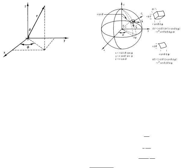
FIGURE L.1. Spherical coordinates.
It is possible to use coordinate systems other than the rectangular (or Cartesian) (x, y, z): In spherical coordinates (Fig. L.1) the coordinates are radius r and angles θ and φ:
x = r sin θ cos φ,
y = r sin θ sin φ, |
(L.1) |
z = r cos θ.
In Cartesian coordinates a volume element is defined by surfaces on which x is constant (at x and x + dx), y is constant, and z is constant. The volume element is a cube with edges dx, dy, and dz. In spherical coordinates, the cube has faces defined by surfaces of constant r, constant θ, and constant φ (Fig. L.2). A volume element is then
dV = (dr)(r dθ)(r sin θ dφ) = r2 sin θ dθ dφ dr. (L.2)
To calculate the divergence of vector J, resolve it into components Jr , Jθ , and Jφ, as shown in Fig. L.2. These components are parallel to the vectors defined by small displacements in the r, θ, and φ directions. A detailed
FIGURE L.2. The volume element and element of surface area in spherical coordinates.
calculation1 shows that the divergence is
div J = · J = |
1 ∂ |
(r2Jr ) + |
1 ∂ |
(sin θ Jθ ) |
||||||||
|
|
|
|
|
|
|||||||
r2 ∂r |
r sin θ |
∂θ |
||||||||||
|
1 ∂ |
|
|
|
|
|
|
|
(L.3) |
|||
+ |
|
|
|
(Jφ). |
|
|
|
|
||||
r sin θ |
∂φ |
|
|
|
|
|||||||
The gradient, which appears in the three-dimensional di usion equation (Fick’s first law), can also be written in spherical coordinates. The components are
∂C ( C)r = ∂r ,
1 ∂C
( C)θ = r ∂θ , (L.4)
1 ∂C
( C)φ = r sin θ ∂φ .
1H. M. Schey (2005). Div, Grad, Curl, and All That. 4th. ed. New York, Norton.
578 Appendix L. Spherical and Cylindrical Coordinates
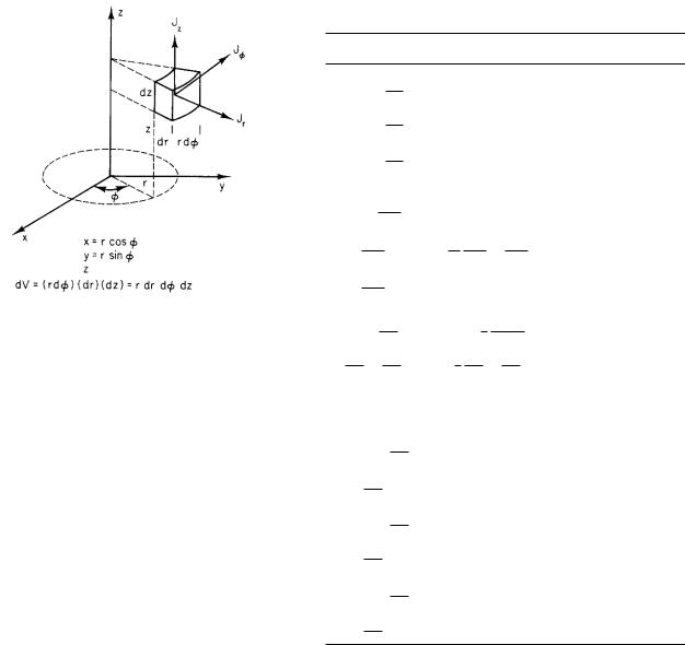
FIGURE L.3. A cylindrical coordinate system.
Figure L.2 also shows that the element of area on the surface of the sphere is (r dθ)(r sin θ dφ) = r2 sin θ dθ dφ. The element of solid angle is therefore
dΩ = sin θ dθ dφ.
This is easily integrated to show that the surface area of a sphere is 4πr2 or that the solid angle is 4π sr.
S = r2 |
π sin θ dθ |
2π dφ = 2πr2 |
π sin θ dθ |
|
0 |
0 |
0 |
= 2πr2 [− cos θ]0π = 4πr2. |
|
||
Similar results can be written down in cylindrical coordinates (r, φ, z), shown in Fig. L.3.
Table L.1 shows the divergence, gradient and curl in rectangular, cylindrical, and spherical coordinates, along with the Laplacian operator 2.
TABLE L.1. The vector operators in rectanguar, cylindrical and spherical coordinates.
Rectangular, |
Cylindrical |
Spherical |
x, y, z |
r, φ, z |
r, θ, φ |
Gradient
( C)x = ∂C ∂x
( C)y = ∂C ∂y
( C)z = ∂C ∂z
Laplacian
2C = ∂2C ∂x2
+ ∂2C ∂y2
+ ∂2C ∂z2
Divergence
· j = ∂jx
∂x
+∂jy + ∂jz ∂y ∂z
Curl
( × j)x = ∂jz
∂y
−∂jy ∂z
( × j)y = ∂jx
∂z
−∂jz ∂x
( × j)z = ∂jy
∂x
−∂jx ∂y
|
( C)r = |
∂C |
|||||||||||
|
|
|
|
|
|
|
|
||||||
|
|
∂r |
|||||||||||
|
( C)φ = |
1 ∂C |
|||||||||||
|
|
|
|
|
|
|
|
||||||
|
r ∂φ |
||||||||||||
|
( C)z = |
|
∂C |
||||||||||
|
|
|
|
|
|||||||||
|
|
∂z |
|||||||||||
2 |
|
1 ∂ |
|
|
∂C |
||||||||
|
C = |
|
|
|
|
|
|
r |
|
|
|||
r |
∂r |
|
|
∂r |
|||||||||
|
1 ∂2C |
|
|
∂2C |
|||||||||
+r2 ∂φ2 + ∂z2
· j = 1 ∂(rjr ) r ∂r
+1 ∂jφ + ∂jz
r ∂φ |
∂z |
|
|
|
( C)r = |
|
|
∂C |
|||||||||||||||||||||||
|
|
|
|
|
|
|
|
|
|
|
|
|
|
|
|||||||||||||||
|
|
|
|
|
∂r |
||||||||||||||||||||||||
|
|
( C)θ = |
1 ∂C |
||||||||||||||||||||||||||
|
|
|
|
|
|
|
|
|
|
|
|
|
|
||||||||||||||||
|
|
r ∂θ |
|||||||||||||||||||||||||||
|
( C)φ = |
|
|
|
|
1 |
|
|
|
∂C |
|||||||||||||||||||
|
|
|
|
|
|
|
|
|
|
|
|
|
|
|
|||||||||||||||
r sin θ |
∂φ |
||||||||||||||||||||||||||||
2 |
|
|
|
|
|
|
1 |
|
|
|
∂ |
|
|
|
|
2 ∂C |
|||||||||||||
|
C = |
|
|
|
|
|
|
|
|
|
|
|
|
r |
|
|
|
|
|
|
|
||||||||
r2 |
∂r |
|
|
|
|
|
∂r |
||||||||||||||||||||||
+ |
|
1 |
|
|
|
|
|
∂ |
sin θ |
∂C |
|
||||||||||||||||||
|
r2 sin θ ∂θ |
|
|
|
|
|
|
|
|
|
|
∂θ |
|||||||||||||||||
|
|
+ |
|
|
|
|
1 |
|
|
|
|
|
|
|
∂2C |
||||||||||||||
|
|
r |
2 |
sin |
2 |
|
|
|
|
|
|
|
2 |
|
|
|
|
|
|||||||||||
|
|
|
|
|
|
|
|
|
θ ∂φ |
||||||||||||||||||||
|
· j = |
|
|
1 ∂(r2jr ) |
|||||||||||||||||||||||||
|
r2 |
|
|
|
|
|
|
∂r |
|
||||||||||||||||||||
|
|
1 |
|
|
|
|
|
∂(sin θjθ ) |
|||||||||||||||||||||
+ |
|
|
|
|
|
|
|
|
|
|
|
|
|
|
|
|
|
|
|
|
|
|
|
|
|
|
|
||
r sin θ |
|
|
|
|
|
∂θ |
|||||||||||||||||||||||
|
|
|
|
|
|
|
|
||||||||||||||||||||||
|
|
+ |
|
|
1 |
|
|
|
|
|
∂jφ |
||||||||||||||||||
|
|
|
|
|
|
|
|
|
|
|
|
|
|
|
|
|
|
|
|
|
|
|
|
|
|
||||
r sin θ ∂φ
( × j)r = |
1 ∂jz |
|
( × j)r = |
|
1 |
|
|
|
||||||||||||||||||||||||
r |
|
∂φ |
|
|
r sin θ |
|
||||||||||||||||||||||||||
− |
∂jφ |
|
× |
|
∂(sin θ jφ) |
|
− |
|
∂(jθ ) |
|||||||||||||||||||||||
|
|
∂z |
|
|
|
|
|
|
|
|
|
|
|
∂θ |
|
|
∂φ |
|
||||||||||||||
( × j)φ = |
∂jr |
|
|
( × j)θ = |
|
1 |
|
|
|
|||||||||||||||||||||||
∂z |
|
|
r sin θ |
|||||||||||||||||||||||||||||
|
|
∂jz |
|
|
∂jr |
|
sin θ∂(rjφ) |
|||||||||||||||||||||||||
− |
|
|
|
|
|
|
|
|
× |
|
|
|
|
|
− |
|
|
|
|
|
|
|||||||||||
|
∂r |
|
|
|
∂φ |
|
|
∂r |
||||||||||||||||||||||||
( × j)z = |
1 ∂(rjφ) |
|
|
|
|
|
|
( × j)φ |
|
|
|
|
|
|||||||||||||||||||
r |
|
|
∂r |
|
|
|
|
|
|
|
|
|
|
|
||||||||||||||||||
1 ∂jr |
|
|
|
|
1 ∂(rjθ ) |
|
|
∂jr |
||||||||||||||||||||||||
− |
|
|
|
|
= |
|
|
|
|
− |
|
|
|
|||||||||||||||||||
r |
∂φ |
r |
∂r |
|
∂θ |
|||||||||||||||||||||||||||

Appendix M
Joint Probability Distributions
In both physics and medicine, the question often arises of what is the probability that x has a certain value xi while y has the value yj . This is called a joint probability. Joint probability can be extended to several variables. This appendix derives some properties of joint probabilities for discrete and continuous variables.
M.1 Discrete Variables
Consider two variables. For simplicity assume that each can assume only two values. The first might be the patients health, with values healthy and sick ; the other might by the results of some laboratory test, with results normal and abnormal. Table M.1 shows the values of the two variables for a sample of 100 patients. The joint probability that a patient is healthy and has a normal test result is P (x = 0, y = 0) = 0.6; the probability that a patient is sick and has an abnormal test is P (1, 1) = 0.15. The probability of a false positive test is P (0, 1) = 0.20; the probability of a false negative is P (1, 0) = 0.05.
The probability that a patient is healthy regardless of the test result is obtained by a summing over all possible test outcomes: P (x = 0) = P (0, 0) + P (0, 1) = 0.6 + 0.2 = 0.8.
In a more general case, we can call the joint probability P (x, y), the probability that x has a certain value
FIGURE M.1. The results of measuring two continuous variables simultaneously. Each experimental result is shown as a point.
independent of y Px(x), and so forth. Then
Px(x) = y |
P (x, y) |
|
(M.1) |
Py (y) = x P (x, y).
TABLE M.1. The results of measurements on 100 patients showing whether they are healthy or sick and whether a laboratory test was normal or abnormal.
Normal test (y = 0) |
Healthy (x = 0) |
Sick (x = 1) |
60 |
5 |
|
Abnormal test (y = 1) |
20 |
15 |
Since any measurement must give some value for x and y, we can write
|
|
|
1 = x Px(x) = |
x y |
P (x, y), |
|
|
(M.2) |
1 = y Py (y) = y x P (x, y).