Добавил:
Опубликованный материал нарушает ваши авторские права? Сообщите нам.
Вуз: Предмет: Файл:

Intermediate Physics for Medicine and Biology - Russell K. Hobbie & Bradley J. Roth

.pdf
Скачиваний:
93
Добавлен:
10.08.2013
Размер:
20.85 Mб
Скачать
= 0.137 (ratio of x rays emitted)

492 17. Nuclear Physics and Nuclear Medicine

17.6.6 Activity per Unit Mass

It is sometimes convenient to use the mean initial activity per unit mass

Ch =

Ah


Bq kg1


(17.45)

mh


and the cumulated mean activity per unit mass


˜

τhA0


˜

Ah

1


Ch =

mh

=


mh

kg


.

(17.46)

Earlier units for these were µCi g1 and µCi h g1.

17.7Mean Energy Emitted per Unit of Cumulated Activity

The mean energy emitted per unit cumulated activity ∆i is determined by knowing ni and Ei for each particle or photon that is emitted. For a given nuclear transformation, the ni and Ei must include all photons (whether γ rays or x rays) and all electrons (betas, internal conversion electrons, and Auger electrons). In SI units,

i (in J) = niEi (in J).

(17.47a)

If Ei is expressed in MeV, we must use the conversion factor 1 MeV = 1.6 ×10¹³ J. In the old system of units, there is the conversion factor:

i (g rad µCi1 h1) = niEi (MeV)

×(3.7 × 10⁴ s1 µCi1)(1.6 × 10¹³ J MeV1)

×(107 erg J1)(3.6 × 10³ s h1)(102 rad g erg1)

i = 2.13niEi.

(17.47b)

Values of ∆i in the old units are found in the “output tables” for each nucleus (see Figs. 17.4, 17.9, and 17.10). We will calculate some values in this section to show how it is done.

Although β particles have a complicated energy spectrum, they are the easiest radiation for which to determine ∆i. Values of ni are available in nuclear data tables that show the decay schemes for the nucleus under consideration, and average β energies have usually been measured. For positron decay, there are also two 0.511-MeV annihilation photons to be considered.

Referring to 18F, Fig. 17.10, we see that 0.97 of the decays are positron emission with an average energy of 0.2496 MeV = 4.00 × 10¹⁴ J. Therefore, ∆i is 0.97 × 4.00 ×1014 = 3.87 ×10¹⁴ J. For the old units, multiply by 2.13/1.6 × 1013 = 1.33 × 10¹³, to get ∆i = 0.516 g rad µCi1 h1, which agrees with the entry under output data of Fig. 17.10. There are two annihilation photons for each nuclear transition, so ni = 1.94 and Ei = 0.511 MeV for the annihilation radiation. This gives ∆i = 1.59 × 10¹³ J or 2.11 g rad µCi1 h1.

TABLE 17.2. Additional properties of 9943Tc for calculation of ∆i.

Fluorescence yielda

WK

0.74

K-shell binding energyb

BK

0.021 04 MeV

L-shell binding energy

BL

0.0028 MeV

M -shell binding energy

BM

0.0005 MeV


Kα

= 0.863 (ratio of x rays emitted)

Kα + Kβ


Kβ

Kα + Kβ

aEstimated using Fig. 17.14.

bBinding energies are from Handbook of Chemistry and Physics, 51st ed., Cleveland, The Chemical Rubber Co., 1966, p. E-186.

Since electron capture competes with positron emission, it is also listed in the input data for 18F as occurring 3% of the time. Most of the energy is taken away by the neutrino, and it does not contribute to the absorbed dose. The x rays emitted by the residual 18O have such low energies that they are not listed in the output data. For a nucleus of higher Z, however, they would be important.

We turn now to γ emission, which often occurs after β emission because the resulting nucleus is not in its ground state. Internal conversion competes with the γ emission. Let us use the specific example 9943mTc, whose decay scheme is shown in Fig. 17.4. The 6-h half-life is associated with a metastable state, and the decay produces three possible γ rays. The “ground state” is actually not stable, but decays by emission with a half-life of 2.1 ×10⁵ yr. The problems will show that this can be neglected.

In addition to the data in the “input data” table of Fig. 17.4, we need some information about the x-ray characteristics of 99Tc. These are listed in Table 17.2. The subscripts of ni, Ei, and ∆i in the following all refer to the line in the output data of Fig. 17.4.

Consider γ1. Its energy (0.0021 MeV) is less than the binding energy of either a K or L electron, so there is no K or L internal conversion. However, αM is very large, and we will assume that all of the γ1 transitions are M -shell internal conversions. In the output table (Fig. 17.4), this means that ∆1 for γ1 is zero. The energy of the internal-conversion electron is the decay energy minus BM : E2 = 0.0021 0.0005 = 0.0016 MeV. Then

2 = n2E2 = (0.9860)(0.0016)(1.6 × 10¹³) = 2.52 × 10¹⁶ J.

The remaining 0.0005 MeV is taken care of by M Auger electrons.

Now consider γ2. There can be γ rays of this energy and internal conversion electrons from the K, L, or M shells. We are told (input data) that αK = 0.104, and that αK = 7.7αL. It is also known empirically that

an electron falls to a hole in the K shell from the L shell

αL 3αM . Therefore, we can write

αK = 0.104, αL = 0.0135, αM = 0.0045.

Now Eq. 17.10 combined with the definition of α gives

fr + αK fr + αLfr + αM fr = 1, fr (1 + αK + αL + αM ) = 1,

1

fr = 1.122 = 0.8913, (17.48) fK = αK fr = 0.0927,

fL = αLfr = 0.0120, fM = αM f r = 0.0040.

Each of these must be multiplied by nγ2 = 0.9860 to get the overall number of photons or internal-conversion electrons per decay associated with γ2:

n3 = nγ2 fr = (0.9860)(0.8913) = 0.8788,

n4 = nγ2 fK = (0.9860)(0.0927) = 0.0914,

(17.49)

n5 = nγ2 fL = (0.9860)(0.0120) = 0.0118,

n6 = nγ2 fM = (0.9860)(0.0040) = 0.0039.

The energies are calculated as follows:

E3 = Eγ2 = 0.1405 MeV,

E4 = Eγ2 − BK = 0.1405 0.0210 = 0.1195 MeV,

E5 = Eγ2 − BL = 0.1405 0.0028 = 0.1377 MeV,

E6 = Eγ2 − BM = 0.1405 0.0005 = 0.1400 MeV.

(17.50)

The values of ∆i are the products of these:

3 = 1.976 × 10¹⁴ J = 0.2627 g rad µCi1 h1,

4 = 1.748 × 10¹⁵ J = 0.0232 g rad µCi1 h1,

5 = 2.600 × 10¹⁶ J = 0.0035 g rad µCi1 h1,

6 = 8.736 × 10¹⁷ J = 0.0012 g rad µCi1 h1.

17.8 Calculation of the Absorbed Fraction

493

The table gives 0.0662 for this sum. Considering that our value of WK was obtained independently of the table, this is good agreement. For Kβ x rays, we get n13 = (0.1001)(0.74)(0.137) = 0.0101. The energies of the x rays are obtained by subtracting the binding energies:

E11(Kα1 ) = BK − BL = 0.0210 0.0028 = 0.0182 MeV,

E13(Kβ ) = BK − BM = 0.0210 0.0005 = 0.0205 MeV.

Of the holes in the K shell, a fraction 1 − WK = 0.26 decay by emission of Auger electrons. The total number of K holes is 0.1001; the total number of K Auger electrons should therefore be (0.1001)(0.26) = 0.0260. The notation of the “output data” table is of the form

KLM

with the emission of an Auger electron from the M shell

The sum of ni for KLL and KLX (X denoting shells above the L shell) is 0.0207, in good agreement with the 0.0260 we calculated.

17.8Calculation of the Absorbed Fraction

The remaining part of the dose determination problem is the most di cult: the calculation of φ(rk ← rh), the fraction of the radiation of a certain type emitted in region rh that is absorbed in region rk . A lot has been published on this problem; this section provides only an introduction.

17.8.1Nonpenetrating Radiation

The simplest case is for charged particles or photons of very low energy that lose all their energy after traveling a short distance. If the source volume is much larger than this distance, we can say that the target volume is the same as the source volume:

φ(rk

rh) =

0,

rk =rh

(17.51)


1

rk = rh.


Similar calculations for the third γ ray are left to the problems.

We must next consider x-ray and Auger electron emission. A K-shell hole can be produced by a K internalconversion electron from either γ2 (n4 = 0.0913) or γ3 (n8 = 0.0088). The total number of holes per nuclear transition is 0.1001. Of these, a fraction WK = 0.74 give x rays. The total number per transition is 0.074. Of these, a fraction Kα/(Kα + Kβ ) = 0.863 go to Kα x rays. These are listed as lines 11 and 12 in the output data of Fig. 17.4. Our calculation gives n11 + n12 = 0.0639.

17.8.2Infinite Source in an Infinite Medium

Suppose that a radioactive source is distributed uniformly throughout a region that is so large that edge e ects can be neglected. The activity per unit mass is C, so the total

˜ ˜

activity is A = M C, where M is the mass of the material.

˜

The energy released is A∆.

This is absorbed in mass M , so the fractional absorbed

energy is 1, as in case 1. The dose is


˜

˜


M C


D =


= C.

(17.52)

M


494 17. Nuclear Physics and Nuclear Medicine

and

Φ =

µen


eµattenr

B(r).

(17.56)


ρ 4πr2


The buildup factor has been tabulated for photons of various energies in water [Berger (1968)].

FIGURE 17.12. A small volume of absorbing material is introduced at distance r from a point source of γ rays.

(This is why ∆ used to be called the equilibrium absorbed dose constant.)

17.8.3Point Source of Monoenergetic Photons in Empty Space

Another simple case is a point source of monoenergetic photons in empty space. The total amount of energy re-

˜

leased by the source is Ai. If the energy of the radiation

˜

is Ei, the number of photons is Ai/Ei. At distance r the

˜ 2

number per unit area is Ai/4πr Ei. If a small amount of substance of area dS, density ρ, thickness dr, and energy absorption coe cient µen is introduced as in Fig. 17.12, the amount of energy absorbed in it is Ei times the


˜


2

.

number of photons absorbed: δE = AidS µendr/4πr


Therefore, the absorbed fraction is


φ =

δE

=

µen dr dS

(17.53)


.

˜

4πr

2


Ai


This is exactly what we expect from the definition of φ. If the source radiates its energy isotropically, the fraction passing through dS is dS/(4πr2). The fraction of that energy absorbed in dr is µen dr. The specific absorbed fraction is

Φ =

φ

=


φ

=


µen


.

(17.54)

M

ρdSdr

4πr2


ρ


17.8.4 Point Source of Monoenergetic Photons

in an Infinite Isotropic Absorber

If the source is not in empty space but in an infinite, homogeneous, isotropic absorbing medium, the number of photons at distance r from the source is modified by the factor e−µattenr B(r), where the buildup factor B(r) accounts for secondary photons. Therefore,

φ =

µen dr dS eµattenr

B(r)

(17.55)


4πr2


17.8.5More Complicated Cases—the MIRD Tables

For more realistic geometries, the calculation of φ is quite complicated. Tables for humans of average build have been prepared by the MIRD Committee [Snyder et al. (1969, 1975, 1976)]. A “Monte Carlo” computer calculation was used. The description below shows how it works in principle; the actual calculations, though equivalent, are di erent in detail to save computer time.

The radioactive nuclei are assumed to be distributed uniformly throughout the source organ. A point within the source organ is picked. The model emits a photon of energy E in some direction, picked at random from all possible directions. This photon is followed along its path; for every element ds of its path, the probability of its interacting, µattends, is calculated. The computer program then “flips a coin” with this probability of having heads. If a head occurs, the photon is considered to interact at that point. If the interaction is Compton scattering, the angle is picked at random with a relative probability given by the di erential cross section. The energy of a recoil electron for that scattering angle is calculated and deposited at the interaction site. Similar procedures are followed for the photoelectric e ect and pair production. The scattered photon is then followed in the same way. If a tail occurred on the first flip, the photon is allowed to travel another distance ds and the probability of interaction is again calculated. This procedure is repeated until all the energy has been absorbed.

To determine what kind of material the photons are traveling through, a model of the body called a phantom is used. An example of a phantom is shown in Fig. 17.13. This entire procedure is repeated many times for each organ, until one has a map of the radiation deposited in all organs by γ rays leaving that point in the source organ.

The procedure is described in much greater detail by Snyder et al. (1969, 1976). Table 17.3 shows a portion of a table for φ. Note that for each photon energy there are two columns: φ and 100σφ, which is the percent fractional standard deviation in φ, related to the square root of the number of photons absorbed in the target organ.

A computer code (OLINDA/EXM) is usually used to make the calculations [Stabin et al. (2005)].

Arqueros and Montesinos (2003) provide a pedagogical discussion of Monte Carlo simulation of γ-ray transport. A pedagogical program for whole-body Monte Carlo calculations has been developed by Hunt et al. (2004). It is

FIGURE 17.13. The phantom used by the MIRD Committee for calculations of the absorbed fraction. (a) A view of the whole body. (b) Details of the heart boundaries. Reprinted by permission of the Society of Nuclear Medicine from W. S. Snyder, M. R. Ford, G. G. Warner, and H. L. Fisher. MIRD Pamphlet No. 5. Estimates of Absorbed Fractions for Monoenergetic Photon Sources Uniformly Distributed in Various Organs of a Heterogeneous Phantom. J. Nucl. Med. 1969; 10 (Suppl. 3): 5–52, Figs. 4 and 5.

available through the RADAR web site: www.doseinforadar.com.

Often most of the isotope is taken up in one or two organs, and the rest of it distributes fairly uniformly through the rest of the body. Using the subscript h for the organs with the greatest activity, TB to mean total

body, and RB to mean the rest of the body,


A˜RB = A˜TB

h


(17.57)


A˜h.


The dose is then


Dk = A˜hS(rk

rh) + A˜RBS(rk

RB).

(17.58)

h


The quantity S(rk RB) cannot easily be tabulated, since it depends on what organs are included in the sum over h. Substituting the tabulated quantity S(rk TB) introduces errors because the “hot” organs that have significant activity are included a second time. One solution to this problem is to modify the cumulated activities [Coffey and Watson (1979)]. First, define a uniform total body cumulated activity that has the same cumulated activity per unit mass as the rest of the body:

˜

mTB

˜


Au =

mRB

ARB.

(17.59)

This activity in the total body would give a dose

˜

Dk = AuS(rk TB).

17.9 Radiopharmaceuticals and Tracers

495

˜ Then define for each organ of interest the quantity Ah,

which is the di erence between the actual activity in organ h and that assuming the substance is uniformly distributed in the total body:


A˜

= A˜

mh

A˜


.


(17.60)


h


h mRB RB


Then the dose to organ k is


Dk =


A˜ S(rk

rh) + A˜uS(rk

TB).

(17.61)


h

h


Problem 32 shows that Eqs. 17.59–17.61 are consistent with Eqs. 17.57 and 17.58 if

mRB

mh

mTB

S(rk RB) +


mTB

S(rk ← rh) = S(rk TB),


h

(17.62)

˜

which is consistent with a uniform source Au distributed throughout the body. The dose can be determined either by calculating the modified activities and using the total body S in Eq. 17.61, or by calculating S for the rest of the body from Eq. 17.62 and using the unmodified activities. Problem 33 shows how these reformulations work in a simple case.

17.9Radiopharmaceuticals and Tracers

A radioactive nucleus by itself is not very useful. It must usually be attached to some substance that will give it the desired biological properties, for example, to be preferentially absorbed in the region of interest. It must also be prepared in a sterile form, free of toxins that produce a fever (pyrogens) so that it can be injected in the patient. This section surveys some of the properties of radiopharmaceuticals.

17.9.1Physical Properties

The half-life must be short enough so that a reasonable fraction of the radioactive decays take place during the diagnostic procedure; any decays taking place later give the patient a dose that has no benefit. (This requirement can be relaxed if the biological excretion is rapid.) On the other hand, the lifetime must be long enough so that the radiopharmaceutical can be prepared and delivered to the patient.

For diagnostic work, the decay scheme should minimize the amount of nonpenetrating radiation. Such radiation provides a dose to the patient but never reaches the detector. This means that there should be as few charged particles (β particles) as possible. The ideal source then is a γ source, which means that the nucleus is in an excited state (an isomer). Such states are usually very short-lived. Not only should the nucleus be a γ emitter, but the internal conversion coe cient should be small, since internal

TABLE 17.3. Absorbed fractions for a uniform source in the lungs, calculated using the MIRD phantom, for photon energies from 10 to 200 keV, with percent errors.


Photon energy


E (MeV)


Target

0.010


0.015


0.020


0.030


0.050


0.100


0.200


Target

organ

φ

100σφ

φ

100σφ

φ


100σφ

φ


100σφ

φ


100σφ

φ

100σφ

φ

100σφ

organ

φ


φ


φ


φ


φ


φ

φ


Adrenals


Bladder


0.124×10³

GI(stomach)


GI(SI)


GI(ULI)


GI(LLI)


0.215×10²

Heart


Kidneys

0.277×10³


0.420×10²

Liver

34

Lungs

0.815

0.27

0.665

Marrow

0.989×10⁴

36

0.234×10²

Pancreas

0.247×10³


0.576×10²

Sk.(rib)

36

Sk.(pelvis)


Sk.(spine)


Sk.(skull)

0.247×10³


0.583×10²

Skeleton

36

(total)


0.209×10³

Skin


Spleen


0.128×10³

Thyroid


Uterus


Trunk

0.996

0.03

0.996

Legs


Head


Total body

0.996

0.03

0.996


0.159×10³

47

0.875×10³

16

0.263×10²


0.170×10³

11

0.983×10²

5

0.228×101


0.142×101


0.326×10³

8.1

4.3

0.258×101

0.39

0.475

0.53

0.231

6.9

0.133×101

2.7

0.386×101


0.312×101


0.379×10³

6.9

2.8

0.710×101


0.128×10²

13

0.148×101


0.331×101


0.264×10³

6.9

2.7

0.952×101

34

0.176×10²

10

0.573×10²

45

0.891×10³

16

0.182×10²

0.03

0.981

0.08

0.875


0.212×10³


0.475×10⁴


35

0.310×10²

0.03

0.981

0.08

0.878

24 0.155×10³

7.8 0.362×10²

340.879×10³

0.294×10³

2.90.203×101

20 0.923×10³

2.90.239×101

0.750.892×101

1.40.466×101

18 0.573×10³

1.60.577×101

0.196×10³

3.80.355×101

26 0.137×10²

1.40.113

4.30.599×102

9.90.205×102

0.383×10⁴

0.180.602

46 0.374×10³

7.40.745×102

0.180.610

19 0.164×10³

0.497×10⁴

5.60.263×102

12 0.137×10²

190.446×10³

0.517×10⁴

2.50.139×101

10 0.901×10³

2.50.173×101

0.970.493×101

1.10.254×101

10 0.607×10³

1.50.243×101

26 0.470×10³

2.30.235×101

11 0.120×10²

1.10.611×101

3.10.541×102

7

0.146×10²

35

0.329×10⁴


0.153×10⁴

0.37

0.384

27

0.390×10³

4.40.793×102

0.370.392

19

0.103 × 10³

24

Adrenals

41

0.145×10³

25

Bladder

5.6

0.250×10²

6.4

GI(stomach)

8.2

0.160×10²

8.2

GI,(SI)

12

0.453×10³

12

GI,(ULI)

31

0.973×10⁴

26

GI(LLI)

2.6

0.130×101

2.9

Heart

8.7

0.934×10³

9.0

Kidneys

2.6

0.155×101

2.8

Liver

1.2

0.498×101

1.4

Lungs

1.4

0.161×101

1.6

Marrow

9.8

0.430×10³

13

Pancreas

1.8

0.145×101

2.3

Sk.(rib)

15

0.348×10³

15

Sk.(pelvis)

2.3

0.153×101

2.7

Sk.(spine)

8.8

0.970×10³

9.7

Sk.(skull)

1.3

0.389×101

1.6

Skeleton (total)

3.1

0.547×10²

3.7

Skin

7.4

0.146×10²

8

Spleen

35

0.539×10⁴

38

Thyroid

47

0.157×10⁴

46

Uterus

0.53

0.351

0.54

Trunk

21

0.427×10³

20

Legs

4.0

0.737×10²

4.0

Head

0.52

0.359

0.53

Total body

Source: Reprinted by permission of the Society of Nuclear Medicine from W. S. Snyder, M. R. Ford, G. G. Warner, and H. L. Fisher. MIRD Pamphlet No. 5. Estimates of Absorbed Fractions for Monoenergetic Photon Sources Uniformly Distributed in Various Organs of a Heterogeneous Phantom. J. Nucl. Med. 1969 10 (Suppl 3): 5–52. Table pp. 30–31, with permission of the publisher.

Medicine Nuclear and Physics Nuclear .17 496

conversion produces nonpenetrating electrons. Positron emitters are more desirable than are βemitters because the positrons produce 0.5-MeV radiation that can reach an external detector. For therapy, on the other hand, nonpenetrating radiation is ideal.

It is also necessary that the decay product have no undesirable radiations. If the decay is a βor β+ decay, the product has di erent chemical properties from the parent and may be taken up selectively by a di erent organ. If it is also radioactive, this can confuse a diagnosis and give an undesirable dose to the other organ.

Ease of chemical separation of the radioactive substance from whatever carrier it is produced with is also important. It is necessary to remove the radioactive isotope from stable isotopes of the same element, because the chemicals are usually toxic. This toxicity is avoided by giving the chemical in minute amounts, which can only be done if the specific activity is high.

17.9.2 Biological Properties

For diagnostic work, a pharmaceutical is needed that is taken up more by the diseased tissue to give a “hot spot” or taken up less to give a “cold spot.” The former is easier to see with small amounts of radioactivity, but both techniques are used. For therapy one wishes to have selective absorption of the pharmaceutical so that the radiations will destroy the target organ but not the rest of the body. There are several mechanisms by which a pharmaceutical may be localized.

1.Active transport. The drug is concentrated by a specific organ against a concentration gradient. Examples are the selective concentration of iodine in the thyroid, salivary, and gastric glands. (It is rapidly excreted from the last two but is retained in the thyroid). This technique is also e ective for certain drugs in the kidney.

2.Phagocytosis. Particles in the size range 1–1,000 nm may be phagocytized—taken up by specialized cells of the reticuloendothelial system. This can take place in liver, bone marrow, and spleen. Particles of size 1 nm go to the Kupfer cells of the liver and to the marrow, while larger particles (100–1,000 nm) are gathered by phagocytes in the liver and spleen.

3.Sequestration. Still larger particles, such as red blood cells that have been denatured by heat, are gathered in the spleen or liver by the process called sequestration. The particles are trapped as the blood percolates through the pulp of the spleen and are later phagocytized.

4.Capillary blockade. The capillaries have a diameter of 7-10 µm. Particles from 20 to 40 µm diameter injected into a vein will find progressively larger vessels as they work their way through the right heart and will be stopped in the capillaries of the lung.

17.9 Radiopharmaceuticals and Tracers

497

FIGURE 17.14. A 99Mo–99mTc generator system. Molybdenum is trapped in the aluminum oxide layer. Eluant introduced at the top flows through and is collected at the bottom.

5.Di usion. It is also possible for a pharmaceutical to move through a membrane to a region of lower concentration. There is a blood–brain barrier between the blood and the central nervous system that is relatively impermeable even to small ions. In a brain scan the chemical is not concentrated in normal brain tissue but leaks into tissue where the blood–brain barrier is compromised by a lesion.

6.Compartmental localization. A suitable pharmaceutical injected in the blood may remain there a long time, mixing well and allowing the blood volume to be determined.

The most widely used isotope is 99mTc. As its name suggests, it does not occur naturally on earth, since it has no stable isotopes. We consider it in some detail to show how an isotope is actually used. Its decay scheme has been discussed above. There is a nearly monoenergetic 140-keV γ ray. Only about 10% of the energy is in the form of nonpenetrating radiation. The isotope is produced in the hospital from the decay of its parent, 99Mo, which is a fission product of 235U and can be separated from about 75 other fission products. The 99Mo decays to 99mTc.

Technetium is made available to hospitals through a “generator” that was developed at Brookhaven National Laboratories in 1957 and is easily shipped. Isotope 99Mo, which has a half-life of 67 h, is adsorbed on an alumina substrate in the form of molybdate (MoO24). From 8 to 100 GBq of 99Mo can be provided. The heart of such a generator (without the lead shielding) is shown in Fig. 17.14. As the 99Mo decays, it becomes pertechnetate (TcO4 ). Sterile isotonic eluting solution is introduced under pressure above the alumina and passes through after filtration into an evacuated eluate container. After removal of the technetium, the continued decay of 99Mo causes the 99mTc concentration to build up again. A generator lasts about a week.

498 17. Nuclear Physics and Nuclear Medicine

Several steps must be taken to prepare the pertechnetate as a radiopharmaceutical. First, it must be checked for breakthrough of the 99Mo. The Nuclear Regulatory Commission allows 1.5 × 10⁴ Bq of 99Mo per Bq of 99mTc. The purity is checked by placing the eluate in a lead sleeve that attenuates the 99mTc γ ray much more than the 750-keV γ rays from 99Mo and measuring the activity. It is also checked with a colorimetric test for the presence of aluminum ion.

The eluate can be used directly for imaging brain, thyroid, salivary gland, urinary bladder, and blood pool, or it can be combined with phosphate, albumin or aggregated albumin, colloidal sulfur, or FeCl3. Commercial kits are available for making these preparations.

For example, kits for labeling aggregated human albumin are commercially available. A vial containing 10 ml of saline solution is enough for ten doses. The aggregated albumin particles are 10–70 µm in diameter. Each milliliter of solution contains (4 8) ×105 particles. Tin is attached to the microspheres and serves to bind technetium. Up to 109 Bq of technetium pertechnetate is added to the vial by the user. A typical adult dose is 10–40 MBq (3.51 ×10⁵ albumin particles). The problems consider attaching Tc to the microspheres and what fraction of the capillaries are blocked by this kind of study.

Other common isotopes are 201Tl, 67Ga, and 123I. Thallium, produced in a cyclotron, is chemically similar to potassium and is used in heart studies, though it is being replaced by 99mTc–sestamibi and 99mTc–tetrofosmin. Gallium is used to image infections and tumors. Iodine is also produced in a cyclotron and is used for thyroid studies.

17.10 Sample Dose Calculation

We pull this discussion together by making a simplified calculation of the dose to various organs from 99mTclabeled microspheres used in a lung scan. We assume that 37 MBq of 99mTc is injected, that it all lodges in the capillaries of the lung, and that it remains there long enough so that the half-life is the physical half-life.9 The residence time is then τh = 1.443T1/2 = (1.443)(6) =


˜

7

8.658 h, so the cumulated

activity is A

lung = (3.7

× 10 )

12

Bq s.

(8.658 × 60 × 60) = 1.153 × 10


The steps in calculating S and the dose are summarized in Table 17.4, which combines information on ∆i with values of φ for lung, heart, liver, head, and the whole body. The values of ∆i are from Fig. 17.15, which is a more

9The last is not a good assumption. The 99mTc leaches from the microspheres into the general circulation. A more accurate calculation requires measurements and the use of a convolution integral, as described in Loevinger et al. (1988, pp. 79–81). The principle residence times are 4.3 h in the lung, 1.8 h in the extravascular space, 0.83 h in the urine, 0.7 h in the kidney, and 0.6 h in the blood.

FIGURE 17.15. The values of ∆i for 99mTc used in Table 17.4 to calculate the dose from a source in the lungs. These are more recent values than those in Fig. 17.4. The reference at the bottom to ruthenium-99 is because 99mTc undergoes β decay in 3.7 × 10⁵ of transitions. This does not a ect any of the entries in the table. Reprinted by permission of the Society of Nuclear Medicine from D. A. Weber, K. F. Eckerman, L. T. Dillman, and J. C. Ryman. MIRD: Radionuclide Data and Decay Schemes. New York, Society of Nuclear Medicine, 1989: 178–179.

recent version of the output table of Fig. 17.4. Table 17.4 refers to the line number for the entry in both Fig. 17.15 and Fig. 17.4. It is worth taking time to compare the entries with the lines in Fig. 17.4 to see the variations with more recent information. Values of φi(rk ← rh) are taken to be 1 in the lung and the whole body when the radiations are nonpenetrating, that is, photons with energy less than 25 keV or electrons. For the high-energy photons (line 3) the values of φ are obtained by interpolation to 140 keV from the values in Table 17.3 for 100 and

200 keV. The sum Sk = ∆iφi, the mass of each organ, and the dose for the cumulated activity of 1.153×10¹² Bq

TABLE 17.4. Values of ∆i, Ei, and φi for 99mTc in the lung.


i (Gy kg1


φi


i,

Ei (keV) (e


Line

i (g

Lung

Heart

Liver

Head

Whole Body

Line

Bq1 s1)

denotes an


in

rad

in


electron)


Fig.

µCi1

Fig.


17.4

h1)

17.15


1 2.56 × 10¹⁶

2 2.64 × 10¹⁷

3 2.00 × 10¹⁴

4 1.70 × 10¹⁵ 5-7 2.15 × 10¹⁶ 8 4.36 × 10¹⁷

98.43 × 10¹⁸

10 1.08 × 10¹⁶ 11-13 3.84 × 10¹⁷

147.64 × 10¹⁸

151.17 × 10¹⁶

166.14 × 10¹⁷

172.26 × 10¹⁷ 18-22 3.419 × 10¹⁷ 23-25 1.623 × 10¹⁷ 26-28 3.367 × 10¹⁷

297.27 × 10¹⁷

iφi

m (kg)

S = ∆iφi/m

Dose (Gy) A0 = 37 MBq


1

0.0000

e

1

0

0

0

1

2

0.0034

e

1

0

0

0

1


0.0004

140.5

0.0495

0.0135

0.0166

0.0077

0.3785

3

0.2670

e

1

0

0

0

1

4

0.0252

e

1

0

0

0

1

5

0.0031

e

1

0

0

0

1

6

0.0006

e

1

0

0

0

1


0.0001

142.6

0.0495

0.0135

0.0166

0.0077

0.3785

7

0.0000

e

1

0

0

0

1

8

0.0014

e

1

0

0

0

1

9

0.0005

e

1

0

0

0

1

10

0.0001

18.37

1

0

0

0

1

11

0.0016

18.25

1

0

0

0

1

12

0.0008

20.62

1

0

0

0

1

13

0.0003

e

1

0

0

0

1

14

0.0005

e

1

0

0

0

1

15

0.0002

e

1

0

0

0

1

16

0.0045

e

1

0

0

0

1

17

0.0010


3.75 × 10¹⁵

2.70 × 10¹⁶

3.32 × 10¹⁶

1.54 × 10¹⁶

1.03 × 10¹⁴


0.999

0.603

1.833

5.278

70.036


3.76 × 10¹⁵

4.48 × 10¹⁶

1.81 × 10¹⁶

2.92 × 10¹⁷

1.48 × 10¹⁶


4.33 × 10³

5.16 × 10⁴

2.09 × 10⁴

3.36 × 10⁵

1.70 × 10⁴


Calculation Dose Sample 10.17

499

500

17. Nuclear Physics and Nuclear Medicine


TABLE 17.5. Some typical doses for nuclear medicine procedures.


Study and agent

A0 (MBq)

Organ and high-

Total body

E ective


est dose (mSv)


dose (mSv)

dose (mSv)


Bone

555

Bladder wall

51

2.0

4.4


99mTc–pyrophosphate


Heart

55

Kidneys

20

3.6

13


201Tl–chloride


Liver

185

Bladder wall

17

0.9

2.6

99mTc–sulfur colloid

Source: Adapted from Table 9-3 in P. B. Zanzonico, A. B. Brill, and D. V.

Becker, Radiation dosimetry, Chapter 9 in H. N. Wagner, Jr., Z. Szabo, and

J. W. Buchanan, eds. Principles of Nuclear Medicine, 2nd. ed. Philadelphia,

Saunders (1995).

s are shown on the bottom lines. The dose to the lungs is 4.3 ×10³ Gy. The whole body dose is much less because the absorbed energy is divided by the mass of the entire body. The value of φ shows that about 38% of the photon energy is absorbed in the body.

The dose to the lungs is considerably greater than in a


chest x ray; however, a chest x ray is almost useless for


diagnosing a pulmonary embolus. The whole body dose


is not unreasonable.


Table 17.5 shows some typical doses from various nu-


clear medicine procedures. The e ective dose is defined

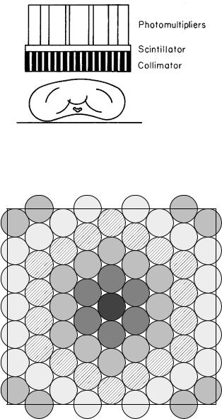
FIGURE 17.16. A scintillator with a lead collimator to give

on p. 468.

directional sensitivity.


17.11 Auger Electrons

is about 4. The fraction of the Auger emitter that binds

to the DNA depends on the chemical agent to which the

In Sec. 15.9 we discussed the deexcitation of atoms, in-

nuclide is attached. There is also a significant bystander

e ect [Kassis (2004)].

cluding the emission of Auger and Coster–Kronig elec-


trons. The Auger cascade means that several of these

17.12 Detectors; The Gamma Camera

electrons are emitted per transition. If a radionuclide is

in a compound that is bound to DNA, the e ect of sev-

Nuclear medicine images do not have the inherent spa-

eral electrons released in the same place is to cause as

much damage per unit dose as high-LET radiation. Lin-

tial resolution of diagnostic x-ray images; however, they

ear energy transfer was defined in Chapter 15. A series of

provide functional information: the increase and decrease

reports on this e ect have been released by the American

of activity as the radiopharmaceutical passes through the

Association of Physicists in Medicine (AAPM) [Sastry

organ being imaged.

(1992); Howell (1992); Humm et al. (1994)].

Early measurements were done with single detectors

Many electrons (up to 25) can be emitted for one

such as the scintillation detector10 shown in Fig. 17.16.

nuclear transformation, depending on the decay scheme

Directional sensitivity is provided by a collimator, which

[Howell (1992)]. The electron energies vary from a few eV

can be cylindrical or tapered. Single detectors are still

to a few tens of keV. Corresponding electron ranges are

used for in vitro measurements and for thyroid uptake

from less than 1 nm to 15 µm. The diameter of the DNA

studies.

double helix is about 2 nm. A number of experiments [re-

Two-dimensional images can be taken with the scin-

viewed in the AAPM reports, also Kassis (2004)] show

tillation camera or gamma camera shown in Figs. 17.17

that when the radioactive substance is in the cytoplasm

and 17.18. The scintillator is 6–12 mm thick and about 60

the cell damage is like that for low-LET radiation in Fig.

cm across. Modern scintillators are rectangular. The scin-

15.32 with relative biological e ectiveness (RBE) = 1.

tillator is viewed by an array of 50–100 photomultiplier

When it is bound to the DNA, survival curves are much

tubes arranged in a hexagonal array. The tube nearest

steeper, as with the α particles in Fig. 15.32 (RBE 8).


When it is in the nucleus but not bound to DNA the RBE

10Scintillation detectors were discussed in Sec. 16.3.

17.13 Single-Photon Emission Computed Tomography

501

FIGURE 17.17. Side view of a scintillation camera. A collimator allows photons from the patient to strike the scintillator directly above the source. An array of photomultiplier tubes records the position and energy of the detected photon.

dahl (1995)]. Some of the aspects of collimator design are discussed in Problems 48–50.

Figure 17.20 shows a bone scan of a child taken with a gamma camera. The 99mTc–diphosphonate is taken up in areas of rapid bone growth. Bone growth at the epiphyses at the end of each bone can be seen. There are also hot spots at the injection site, in one kidney, and in the bladder.

Nuclear medicine can show physiologic function. For example, if the isotope is uniformly distributed in the blood, viewing the heart and synchronizing the data accumulation with the electrocardiogram (gating) allows one to measure blood volume in the heart when it is full and contracted, and to calculate the ejection fraction, the fraction of blood in the full left ventricle that is pumped out. Fig. 17.21, shows pictures and contours of the heart at end-systole and end-diastole. The imaging agent was 99mTc-labeled human red blood cells.

Figure 17.22 shows a series of images taken at six different angles around a patient who has had a lung transplant. The left lung is new and shows considerably more activity than the diseased right lung.

FIGURE 17.18. A square scintillator viewed by an array of 67 photomultiplier tubes. The hexagonal arrangement of the tubes above the scintillator gives the closest spacing between tubes.

where the photon interacts receives the greatest signal. Signals from each tube are combined to give the total energy signal and x and y position signals.

The collimator is a critical component of the gamma camera. The channels are usually hexagonal, with walls just thick enough to stop most of the photons which do not pass down the collimator opening. The collimator usually has parallel channels; single pinholes, diverging, and converging channels are sometimes used and can lead to geometric distortions of the image [Cherry et al. (2003), p. 221, 239 )]. The spatial resolution depends on the distance from the source to the collimator, as shown for one collimator in Fig. 17.19. There are trade- o s between sensitivity and resolution [Links and Eng-

17.13Single-Photon Emission Computed Tomography

Still another detection scheme, single-photon emission computed tomography (SPECT), is analogous to computed tomography (CT). The detector is sensitive to all radioactivity along a line passing through the patient. The counting rate is thus proportional to a projection through the patient, and a cross-sectional slice can be reconstructed from a series of projections, just as was done with x-ray CT using the techniques in Ch. 12. A series of images like those in Fig. 17.22, but at more angles, are used to reconstruct a three-dimensional image that can then be viewed from any direction, with slices at any desired depth. A SPECT scan is shown in Fig. 17.23. There are five reconstructed slices in planes parallel to the long axis of the heart. The left ventricle is prominent, and the right ventricle can be seen faintly in the last few slices.

One of the problems with SPECT is photon attenuation along the projection line. This is shown in Fig. 17.24 for a cylindrical source with uniform activity throughout. Let AV be the activity per unit volume, and ignore variations in 1/r2. The projection F (x) is

a

F (x) = AV (x, y) ∆x z e−µ(y+a) dy, (17.63)

−a

where dy x z is the volume detected. When AV (x, y) is constant (a uniform activity distribution), this can be integrated to give

F =

AV xz

1 − e

2µ(R2

x2)1/2

(17.64)

µ


.