Intermediate Physics for Medicine and Biology - Russell K. Hobbie & Bradley J. Roth

462 16. Medical Use of X Rays

Total Dose (Gy)

FIGURE 16.39. The fraction of cells surviving a total radiation dose when the dose is divided into 1, 2, and 32 fractions, showing how the curve approaches e−αD as the number of fractions becomes large.

What total dose (or dose per fraction) should be given in how many fractions, with what time between fractions? We can answer these questions using the linear-quadratic model. Let the dose per fraction be Df , the number of fractions be n, and the total dose be D = nDf . We now need to plot survival vs total dose for di erent numbers of fractions. We assume that the time between fractions allows for full repair of sublethal damage (single-strand breaks). The probability of a cell surviving after n fractions have been delivered is

Ps = Psurvival = S = e−αDf −βDf2 n = e−αD−βD2/n.

(16.32) As the number of fractions becomes very large for a given total dose, the survival curve approaches e−αD . This can be seen in Fig. 16.39, which plots survival vs total dose delivered in di erent numbers of fractions. With many fractions the dose per fraction is very small, all the singlestrand breaks are repaired, and almost no type-B cell deaths take place.

Early-responding tissue and tumors have been found to have an α/β ratio of about 10 Gy. The survival curve is primarily due to type-A damage. Late-responding tissues have an α/β ratio of 2–3 Gy. There is considerable variation in these numbers.

Some of the problems of radiation therapy and the benefits of fractionation can be seen if we consider a strictly hypothetical example in which α = 0.1 Gy−1 for both the tumor and the surrounding tissue. The tumor is early responding with α/β = 10 Gy, and the surrounding tissue is late responding with α/β = 2 Gy. The surrounding tissue is actually more sensitive to the radiation than the tumor and has a lower survival curve. Figure 16.40 shows the cell-survival curves for 1 and 35 fractions. The tumor survival in each case is shown as a dashed line. The thicker curves correspond to delivering the dose in 35 fractions. (In this example, both tissues have the same value

Total Dose (Gy)

FIGURE 16.40. Cell survival curves for late-responding normal tissue (LRT) and for a hypothetical tumor (T), showing the improvement obtained by dividing the dose into fractions. With a single fraction, the tumor survives much better than the normal tissue. With 35 fractions, this discrepancy has been reduced. The details are discussed in the text.

of α and the surrounding tissue receives the same dose. In real life, α for the tumor may be greater than that for the normal tissue, and the treatment will be more e ective.)

To see the benefit of fractionation, suppose that the patient can tolerate a dose at which only 10−6 of the cells of the surrounding tissue survive, represented by the horizontal line on the graph. (This is not realistic!) For a single fraction, this corresponds to a total dose of about 9 Gy, which, applied to the dashed line, shows that the surviving fraction of tumor cells is about 10−2. For 35 fractions the normal tissue can tolerate about 32 Gy, yielding 3 ×10−5 as the fraction of tumor cells surviving.

Suppose next that it is possible to confine the radiation beam so that the dose to normal tissue is only about 0.6 times that to the tumor. This means that the tissue dose in Eq. 16.32 is multiplied by 0.6. The result is shown in Fig. 16.41 for 35 fractions. The dose can now be as high as 53 Gy for the same e ect on surrounding tissues, leading to a tumor survival of only 10−8. We will see how beam shaping is accomplished in the next section.

These calculations are solely to illustrate the basic principles. Clinically useful calculations must take several additional factors into account: the actual values of α for the tissue and tumor under consideration, the e ect of cell growth after irradiation, the e ect of the first dose on synchronizing the cycles of the remaining cells, and the oxygen level in the tumor cells. (The greater the oxygen concentration the more sensitive the cells are, particularly for low-LET radiation. Rapidly growing tumors often outstrip their blood supply, receive less oxygen, and are less radio-sensitive.) Fractionation is reviewed in Orton (1997) and in Hall (2000). It is also necessary to take into account the fact that neither the tumor nor the surrounding normal tissue receives a uniform dose of radiation.

Dose (Gy)

Dose (Gy)

FIGURE 16.41. Survival curves for the same cells as in the previous figure, with the dose to the surrounding tissue reduced to 0.6 times that to the tumor. Now the probability of tumor survival at high doses is about 0.01 times that for the surrounding normal tissue. This shows the importance of confining the radiation to the tumor as much as possible.

FIGURE 16.43. The probability of curing the tumor and the probability of unacceptable damage to normal tissue vs dose. Both the tumor and the normal tissue contain 108 cells. The 35-fraction doses shown in Fig. 16.41 have been used.

This can be evaluated using your cell-survival model of choice.

Figure 16.42 shows a tumor eradication curve based on the 35-fraction curve in Fig. 16.40. The larger the tumor, the greater the dose required for cure. Figure 16.43 shows a plot of the probability of tumor cure and the probability of unacceptable damage to the surrounding tissue, both based on 108 cells and the cell-survival curves in Fig. 16.41 (with the normal tissue receiving 0.6 times the dose received by the tumor). For this model, at least 60 Gy are required in order to have a good probability of cure; once the dose is higher than 63 Gy, the damage to normal tissue is unacceptable.

Dose (Gy)

FIGURE 16.42. The probability of eradicating the tumor (no surviving tumor cells) as a function of dose for tumors containing di erent numbers of cells.

16.10.6 A Model for Tumor Eradication

The target theory model can be applied to a collection of cells to give us insight into the central problem of radiation therapy: eradication of the tumor or tumor eradication. Suppose that a tumor consists of N cells with identical properties. The cells are uniformly irradiated with dose D. If a collection of identical tumors were irradiated, the number of cells surviving in each tumor would fluctuate. The probability that a single cell survives is ps(D), which might be given by Eq. 16.32. If this number is small and N is large, the number surviving follows a Poisson distribution. The average number surviving is m = N ps(D). The probability of a cure is the probability that no tumor cells survive:

16.11 Radiation Therapy

The treatment of cancer must deal with two issues: eradication of the primary tumor (local control), and eradication of metastases, which may be in nearby tissue or may be at distant sites within the body. In many cases radiation therapy, either alone or combined with surgery, is the best technique for local control. Two oncologists have provided a review of the benefits and problems of radiation therapy, addressed specifically to the medical physics community [Schulz and Kagan (2002)]. They point out that many cancer deaths are due to metastatic disease, so improved local control does not necessarily provide a corresponding improvement in survival.

Which method of treatment is best can change dramatically as new treatments are developed. For example, a combination of radiation therapy and chemotherapy was once used to treat Hodgkin’s disease; chemotherapy has been improved to the point where radiation is no longer necessary [DeVita (2003)].

464 16. Medical Use of X Rays

FIGURE 16.44. X-ray therapy was used to treat a carcinoma of the nose. A shows the original lesion; B is the result one year later. The patient remained asymptomatic five years after treatment. Reprinted from William T. Moss and James D. Cox. Radiation Oncology, 6th ed. (1989) St. Louis, Mosby, with permission from Elsevier.

16.11.1Classical Radiation Therapy

Doses for diagnostic radiology vary from about 10−4 to 10−2 Gy. Doses of 20–80 Gy are required to treat cancer. A great deal of physics is involved in planning the treatment for each patient. [See Khan (2003).] There is a choice of radiation beams: photons of various energies, electrons, neutrons, protons, or α particles. Photons and electrons are routinely available; the other sources require special facilities. Only a few of the beam issues will be raised here. Some of the dose measurement issues are discussed in the next section.

An example of the e ectiveness of radiation therapy is shown in Fig. 16.44 The patient developed a carcinoma of the nose and refused surgery. Radiation with a total dose of 50 Gy was used, and the results one year later are shown. It is ironic that the carcinoma probably developed because the patient was treated with x rays for acne many years earlier.

We have already seen the importance of reducing dose to tissue surrounding the tumor. Optimizing the dose determines the kind of radiation to be used and its energy, as well as the details of beam filtration and collimation and how it is aimed at the patients body. For now, we discuss a photon beam. Attenuation and the 1/r2 decrease of photon fluence help spare tissue downstream from the beam. Since µatten decreases with increasing photon energy up to a few MeV, higher-energy photons penetrate more deeply and must be used for treating deeper lesions. There is also dose buildup with depth over distances comparable to the range of the Compton-scattered electrons. Both of these e ects are shown in Fig. 16.45.

The beam is collimated to spare normal tissue. Originally, the collimator consisted of four lead jaws that provided a rectangular opening with adjustable length and

FIGURE 16.45. The dose vs depth for x-ray beams of di erent quality (energy) on the central axis of the beam. The source— surface distance (SSD) is 100 cm and the field size is 10 cm×10 cm. The curve “3.0 mm Cu HVL” is for a photon beam that is reduced to half intensity by a copper filter 3.0 mm thick. The labels 4, 10 and 25 MV refer to the energy of the electron beam striking the target. From F. M. Khan (2003). The Physics of Radiation Therapy, 3rd. ed. Philadelphia, Lippincott Williams & Wilkins, p.163. c 2003 Lippincott Williams and Wilkins.

width. Later, masks of a special lead alloy were custommade for each patient. A wedge was sometimes placed in the beam to vary the intensity across the collimated radiation field.

Figure 16.46 shows isodose contours for various beams. In addition to the di erences with depth seen in Fig. 16.45, there are significant di erences in the sharpness of the dose distribution across the beam. The extent of the lesion to be radiated must be carefully determined with radiographs or CT scans.

If the tumor is not near the surface, the ratio of tumor dose to normal tissue dose can be increased by irradiating the patient from several directions. Figure 16.47 shows how the relative dose to a deep tumor can be increased by irradiating with two “fields” on opposite sides of the patient. In Fig. 16.48 three and four fields are used. The angles of the fields can be changed by rotating the patient couch as well as the gantry holding the photon source and collimator.

Rectangular fields do not match the shape of the tumor. Two techniques can overcome this problem. A leadalloy that melts at low temperature can be used to make a collimator that is customized for each patient to match the tumor. Or, a multi-leaf collimator can replace the original jaws on the therapy machine. A typical multileaf collimator has 40 pairs of tungsten alloy leaves, each ≤ 1 cm wide, which can be independently adjusted to provide a pattern like that in Fig. 16.49. This might be used for up to nine fields from di erent directions.

FIGURE 16.46. Isodose distributions for radiation under different conditions, all collimated to 10 cm×10 cm. (A) Radiation from an x-ray tube with 200 kVp, 0.5 m from the surface.

(B) Photons from the radioactive isotope 60Co, 0.8 m from the surface. (C) 4-MV photons, 1 m from the surface. (D) 10-MV photons, 1 m from the surface. From F. M. Khan, The Physics of Radiation Therapy, 3rd. ed. p. 204. Philadelphia, Lippincott Williams & Wilkins. c 2003 Lippincott Williams & Wilkins.

16.11.2Modern X-ray Therapy

The goal of radiation therapy is to provide as large a dose as possible to the tumor while sparing adjacent normal tissue. The normal tissue may be quite close to the tumor. Three-dimensional conformal radiation therapy uses 3-dimensional information about the target volume. This is di cult, because even with 3-D display of CT, MRI or ultrasound images, it may be impossible to see the edges of the tumor. Nevertheless, the beam’s-eye view that can be computed from 3-D image data can be very useful in planning the treatment. For a discussion of conformal radiation therapy, see Khan (2003), Chapter 19.

In classical radiotherapy, the beam was either of uniform fluence across the field, or it was shaped by an attenuating wedge placed in the field. Intensity-modulated radiation therapy (IMRT) is achieved by stepping the collimator leaves during exposure so that the fluence varies

FIGURE 16.47. Isodose distribution when the patient is irradiated equally from opposite sides. From F. M. Khan, The Physics of Radiation Therapy, 3rd. ed. Philadelphia, Lippincott Williams & Wilkins. c 2003 Lippincott Williams & Wilkins.

from square to square in Fig. 16.49 [Webb (2001); Khan (2003), Ch. 20]. One form of IMRT is helical tomotherapy (slice therapy), which uses filtered back-projection techniques with a multileaf collimator to shape the radiation field as the patient moves axially through the beam—the analog of a spiral CT study [Holmes et al. (1995)]. It is, of course, impossible to make the filtered radiation field negative. This means that the dose outside the tumor is not strictly zero, but it can be made small. These techniques provide much better sparing of adjacent sensitive tissue and sometimes allow a boost in dose to the tumor. One drawback to IMRT is that although the dose to the tumor is about the same, the total number of x rays produced is a factor of 2–10 greater than in conventional therapy. This requires better-shielded radiation treatment rooms.

16.11.3Charged Particles and Neutrons

Electrons, typically between 6 and 20 MeV, are also used for therapy. Because of the range–energy relationship, the field falls nearly to zero in a centimeter or two. Electrons are used primarily for skin and lip cancer, head and neck cancer, and irradiation of lymph nodes near the surface. Figure 16.50 shows the dose vs. depth as a percent of the maximum dose for electron beams of several di erent energies.

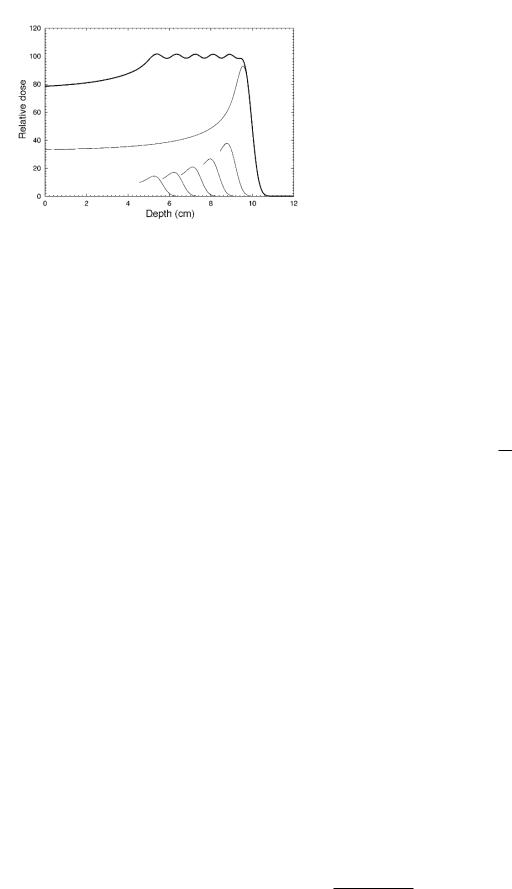
FIGURE 16.52. irradiating the patient through a number of absorbers of di erent thickness spreads out the region of maximum dose. Provided by W. D. Newhauser, M. D. Anderson Cancer Center.

proves more successful and the patients survive longer. Miralbell et al. (2002) estimated the incidence rate for secondary cancers in certain pediatric cancers and found a reduced incidence for proton therapy compared to both conventional x ray and IMRT. Intensity-modulated proton therapy could provide even more improvement.

Proton therapy is used in a number of diseases, such as prostate cancer [Slater et al. (2004)], retinal tumors such as choroidal melanoma, pituitary adenoma, arteriovenous malformations in the brain, and wet macular degeneration [Habrand et al. (1995), Suit and Urie (1992), Moyers (2003)]. Some institutions are experimenting with intensity-modulated proton therapy (IMPT).

Fast neutrons are used for therapy [Duncan (1994)]. The dose is due to charged particles: protons, α particles (4He nuclei), or recoil nuclei of oxygen and carbon that result from interactions of the neutrons with the target tissue. All of these have high LET, and the oxygen e ect is less than for low-LET radiation. Fast neutron therapy shows promise in some salivary gland cancers [Douglas et al. (2003)].

Boron neutron capture therapy (BNCT) is based on a nuclear reaction which occurs when the stable isotope 10B is irradiated with neutrons, leading to the nuclear reaction (in the notation of Chapter 17)

105 B +10 n →42 α +73 Li or 105 B(n, α)73Li.

Both the alpha particle and lithium are heavily ionizing and travel only about one cell diameter. BNCT has been tried since the 1950s; success requires boron-containing drugs that accumulate in the tumor. The field has recently been reviewed by Barth (2003).

Brachytherapy (brachy means short) involves the implantation of radioactive isotopes in a tumor and will be discussed in Chapter 17.

16.12 Dose Measurement

It is important to measure radiation doses accurately for radiation therapy in order to compare the e ectiveness of di erent treatment protocols and to ensure that the desired protocol is indeed being followed. Accuracies of 2% are expected. An extensive literature about relating the dose in the measuring instrument to the dose in surrounding tissue exists.21 Here we describe one of the techniques that is used.

A basic problem in dosimetry is that the measuring instrument has di erent properties than the medium in which it is immersed. Imagine, for example, that a gasfilled ionization chamber is placed in water. If the radiation field were very large and uniform, one could in principle use an ionization chamber whose dimensions are large compared to the range of secondary electrons, and the interaction of the radiation field with the chamber gas would be the dominant e ect. This is not practical. At the other extreme, we imagine an ionization chamber that is so small that it does not alter the radiation field of the water. That is, its dimensions must be small compared to the range of the charged particles created in the water and passing through it.

We saw in Sec. 15.16 that the absorbed dose in a parallel beam of charged particles with particle fluence Φ is (Eq. 15.76)

D = Sρe Φ.

Usually the beam consists of particles with di erent kinetic energies T . Let ΦT be the energy spectrum:

Then the dose is the integral of the number of particles with energy T times the mass stopping power for particles of that energy:

We can define an average mass collision stopping power:

Let us apply this to the situation where a small detector (“gas”) is introduced in a medium (“water”) in which we want to know the dose. The charged particle fluence is not altered by the detector because it is small compared

21See Attix (1986), Chap. 10 or Khan (2003), Chapter 8.

We have already seen that the biological e ect of radiation depends on the absorbed dose, the LET, the nature of the tissue that is irradiated, and the dose rate. It also depends on the age of the subject. This makes it very difficult to estimate the detriment. Ideally, we would multiply the dose to each organ or target in the body by the probability of a detriment to that target from that kind of radiation now and in the future, and sum over all the organs in the body. This is impossible: we do not know enough. We must simplify the problem while taking some of these di erences into account.22

16.13.1Equivalent and E ective Dose

Equivalent Dose

Our first simplification assumes that the LET dependence is the same for all target organs. ICRP defines the radiation weighting factor WR for each radiation type R striking the body. It depends on the radiation type and energy and is independent of organ or tissue type. The radiation weighting factor for x rays is 1. WR is determined “with guidance” from an earlier quantity, the relative biological e ectiveness of the radiation (RBE). The weighting factor for each radiation WR is multiplied by the average dose to the target organ or tissue DR,T and summed to give the equivalent dose23 to the target organ, HT :

HT = WRDR,T . (16.40)

R

The unit of HT is the sievert (Sv).24

Detriment and E ective Dose

16.13 The Risk of Radiation

Exposure to radiation may or may not cause a noticeable e ect. E ects can include a change, which may not be harmful; damage to cells, which may not necessarily be deleterious to the individual; or harm, which is clinically observable in the subject or possibly a descendant (though current data suggest that genetic changes are rare). It may take years before the harm is observed. The International Commission on Radiological Protection in ICRP (1991) defines the detriment to an individual who receives a dose of radiation. It is a rather complex combination of the probabillity of harm, the severity of the harm, and the time of onset after exposure. It will be discussed more below.

In this section we focus on the increased probability of induction of cancer from an exposure to radiation. We have considerably more information about human exposure to ionizing radiation than we have for any other known or suspected carcinogen [Boice (1996)]. Several studies at moderate doses show that radiation is a relatively weak carcinogen, though this is not the public view.

The detriment is a measure of the harm from an exposure to radiation. It might be a genetic e ect (relatively rare) or the development of cancer some years later. If cancer, it might be fatal, shortening life span, or it might cause discomfort and inconvenience but not death. We want to estimate the detriment when a certain equivalent dose has been delivered to some target organs. We assume that

22RKH wishes to thank Cynthia McCullough, PhD, for a very helpful discussion of this section

23The nomenclature here is quite confusing. ICRP used to define the dose equivalent, also denoted by H, as QD, where Q was called the quality factor of the radiation. The radiation weighting factor is very similar, and essentially numerically equivalent, to the earlier quality factor, Q. Values of Q recommended by Nuclear Regulatory Commission (NRC) are 1 for photons and electrons, 10 for neutrons of unknown energy and high-energy protons, and 20 for α particles, multiply charged ions, fission fragments, and heavy particles of unknown charge. The ICRP has its own recommendations, that di er slightly for protons and neutrons. See McCollough and Schueler (2000).

24Both the sievert and the gray are J kg−1. Di erent names are used to emphasize the fact that they are quite di erent quantities. One is physical, and the other includes biological e ects. An older unit for H is the rem. 100 rem = 1 Sv.

TABLE 16.4. Contribution of some organs to the whole-body radiation detriment. From ICRP (1991) Table B-20.

the probability of developing cancer in a target organ depends on the dose to that organ and not on the dose to any other part of the body. We also assume that the probabilities are small, so that if several organs have received a radiation dose, the probability of developing cancer is the sum of the probabilities for each organ.

Most of our information about the detriment comes from extensive studies of atomic-bomb survivors, for whom the entire body received a fairly uniform equivalent dose. These survivors have now been followed for over 50 years. Other studies include patients who have been followed for decades after receiving radiation therapy. ICRP (1991) estimates the radiation detriment using these data and taking into account the probability of a fatal cancer attributable to the radiation, the weighted probability of an attributable non-fatal cancer, the weighted probability of severe hereditary e ects, and the relative decrease in lifespan. Table 16.4 shows four of the 14 entries in Table B-20 of ICRP (1991). The details of the various corrections are not shown; the point is to show how each organ contributes to the total detriment.25

The e ective dose26 E is a sum over all irradiated organs:

TABLE 16.5. Major contributions to the e ective dose from a typical CT head scan.

Equivalent Dose (Sv)

FIGURE 16.53. Various doses on a logarithmic scale. Natural background is per year; other doses are per exposure.

10−3 = 9 × 10−5. If the whole body were to receive an equivalent dose of 36 mSv, the probability of a radiationinduced cancer would be 500 × 10−4 × 36 × 10−3 = 1.8 × 10−3.

16.13.2Comparison with Natural Background

The tissue weighting factor WT is the radiation detriment for organ T from a whole body irradiation as a fraction of the total radiation detriment. By definition, the sum of WT over all organs equals unity. The last column of Table 16.4 shows the WT assigned to each target organ in ICRP (1991). See also the review by McCollough and Schueler (2000).

As an example, consider a typical CT head scan, which provides a significant equivalent dose to the brain, bone marrow, thyroid, and bone surface, as shown in Table 16.5.27 The e ective dose is 1.8 mSv. The probability of developing a radiation-induced cancer is 500×10−4 ×1.8×

25ICRP is expected to issue revised values of WT , probably in 2007.

26An older, related quantity is the e ective dose equivalent, HE =

WT QD.

27Values of HT were provided by C. McColllough.

One way to express risk is to compare medical doses to the natural background. We are continuously exposed to radiation from natural sources. These include cosmic radiation, which varies with altitude and latitude; rock, sand, brick, and concrete containing varying amounts of radioactive minerals; the naturally occurring radionuclides in our bodies such as 14C and 40K; and radioactive progeny from radon gas from the earth.28 In a typical adult, there are about 4 × 107 radioactive disintegrations per hour from all internal sources. Table 16.6 and Fig. 16.53 summarize the various sources of

28Radon is chemically inert gas that escapes from the earth. Since it is chemically inert, we breathe it in and out. When it decays in the air (the decay scheme is described in Sec. 17.16), the decay products attach themselves to dust particles in the air. When we breathe these dust particles, some become attached to the lining of the lungs, irradiating adjacent cells as they undergo further decay.

U.S. population, average e ective dose rate (mSv yr−1)a

aNCRP Report 94 (1987) Table 9.7

TABLE 16.7. Typical radiation equivalent doses for the population of the United States. From NCRP 93.

radiation exposure. The radon entry in Table 16.6 is based on a WR of 20 for α particles from radon progeny, the value used by NCRP.29 There is considerable uncertainty in this determination: WR could be as low as 3, in which case radon would contribute much less to the natural background.

Diagnostic procedures give doses that are in general comparable to the average annual background dose, as can be seen in Table 16.7. The higher CT doses correspond to pediatric CT; see Fig. 16.56. One can explain

29The dose to the lungs from radon progeny is about 1 mGy yr−1. This is multiplied by Wr = 20 and WT = 0.12 (lungs) to arrive at an e ective dose of 2.4 mSv yr−1.

to a patient that a chest x ray is equivalent to about one week of natural background, and a mammogram is equivalent to a month or two. A conventional fluoroscopic study of the lower digestive system is equivalent to about a year of natural background.

16.13.3Calculating Risk

Assessing the risk of radiation is complicated, since a radiation-induced cancer, for example, may not appear for many years. It is therefore necessary to specify how many years one watches a population after exposure, age at exposure, and current age. One also has to specify whether the risk is of acquiring the disease or of dying from it. Whatever criteria we use, we can define a risk r(H) that depends on the equivalent dose. We then define the excess absolute risk

The units of r and excess absolute risk can vary. The risk might be per person per year, or it might be for a certain number of years or for a lifetime exposure. The excess relative risk has the advantage of being dimensionless. It is frequently reported, even though it can

be di cult to understand intuitively. (Plots of EAR vs. dose for breast cancer in Japanese women and women in the United States have nearly the same slope. However, r(0) is smaller for Japanese women, leading to a higher ERR.)

Consider a rare disease, and suppose that the probability of acquiring the disease over a lifetime is 2 × 10−3, while in a population that has received a particular dose of something (which might be radiation, or a chemical, or a particular behavior) the probability is 5 × 10−3. Then the excess absolute risk is 3 × 10−3, while the excess relative risk is 150%. A person hearing that the relative risk has increased by 1.5 times might be unduly alarmed, not realizing that there are only three additional cases in 1,000 people.

Statistical fluctuations can make it quite di cult to measure excess risk. Suppose that we want to determine whether r increases linearly with dose. Measurements at lower doses to determine if the response is linear are difficult to make, requiring large numbers of subjects, as the following simplified example shows. Suppose that we have two measurements of the probability of acquiring cancer: one at zero dose, which gives r(0), the “spontaneous” probability due to nonradiation causes, and one at a fairly large dose (say 0.25 Sv, represented by the vertical dashed line on the right in Fig. 16.54). At some lower dose we want to make a measurement to distinguish between a linear increase of probability with dose and a probability that remains at the “spontaneous” value because we are below some threshold dose for carcinogenicity. The probability p = r(H) of acquiring cancer is small, and the total population N is large. This means that if the experiment could be repeated several times on identical populations, the number of persons acquiring cancer, n, would be Pois-

son distributed with mean number m = N p = N r(H)

√

and standard deviation σ = m. Figure 16.54 plots m vs dose for some value of N , with dotted lines to indicate m ±σ. A measurement at the lower dose indicated by the vertical dashed line on the left will not distinguish between the two curves. The only way to reduce the width between the dotted lines at m±σ would be to use a larger population N .

To be quantitative, suppose that r(H) = e + αH, with e = 0.044 and α = 0.013 Sv−1. At a dose of 0.25 Sv, r = 0.047. For 105 persons, the constant curve (expected in the absence of radiation or below threshold) gives m = 4, 400 ± 66, while the linear curve gives m = 4, 730 ± 69. The two curves are distinguishable. At a dose of 0.01 Sv, m for the constant curve is still 4, 400 ± 66, while for the linear case it is 4, 410 ±66. It is impossible to distinguish between the linear and constant curves.

The Linear Nonthreshold Model and Collective Dose

In dealing with radiation to the population at large, or to populations of radiation workers, the policy of the various regulatory agencies has been to adopt the linear-

FIGURE 16.54. Plot of the average number of cases from a population N for a linear–no-threshold and a constant model. The dashed lines represent the mean ±1 standard deviation.

nonthreshold (LNT) model to extrapolate from what is known about the excess risk of cancer at moderately high doses and high dose rates, to low doses, including those below natural background.

If the excess probability of acquiring a particular disease is αH in a population N , the average number of extra persons with the disease is

The product N H, expressed in person·Sv, is called the collective dose. It is widely used in radiation protection, but it is meaningful only if the LNT assumption is correct. Small doses to very large populations can give fairly large values of m, assuming that the value of α determined at large doses is valid at small doses.

It has been suggested that there may in some cases be a threshold for radiation-induced damage. If there is a threshold, then the LNT model gives an overestimate. The latest reports of expert panels continue to recommend the LNT model [NCRP Report 136 (2001), Upton (2003), BEIR Report VII (2005)], but their recommendation is still questioned [Higson (2004)].

To help put the risk in perspective, consider the following example from BEIR (2005), p. 15. Among 100 people, about 42 will be diagnosed with cancer during their lifetime in the absence of any excess radiation. If they had all received a dose of 0.1 Gy (100 mSv for low-LET radiation), there could be one additional cancer in the group.

Even if the LNT model is correct, it can lead to regulatory decisions which are not reasonable. For example, Brooks (2003) cites a study in which the process of cleaning up several Department of Energy sites resulted in more fatal worker accidents than the number of lives that were calculated to have been saved, based on the LNT model.