

Intermediate Physics for Medicine and Biology - Russell K. Hobbie & Bradley J. Roth
.pdf328 12. Images
This is a two-dimensional convolution. The convolution theorem is
Cimage(kx, ky ) = Cobject(kx, ky )Ch(kx, ky )
−Sobject(kx, ky )Sh(kx, ky ),
(12.15)
Simage(kx, ky ) = Cobject(kx, ky )Sh(kx, ky ) +Sobject(kx, ky )Ch(kx, ky ).
12.2.2Optical-, Modulation-, and Phase-Transfer Functions
The optical transfer function (OTF) is the Fourier transform of the point-spread function, Ch(kx, ky ) and Sh(kx, ky ). It is analogous to the transfer function for an amplifier (Sec. 11.15). The modulation transfer function
(MTF) is the amplitude of the OTF:
FIGURE 12.1. The point-spread function and modulation transfer function for a di raction-limited circular aperture. From C. S. Williams and O. A. Becklund. Optics: A Short Course for Engineers and Scientists. New York, Wiley, 1972. Used by permission of the authors.
MTF(kx, ky ) = Ch2(kx, ky ) + Sh2(kx, ky ) 1/2 . |
(12.16) |
|||
The phase transfer function is |
|
|
||
Sh(kx, ky ) |
|
|
||
PTF(kx, ky ) = tan−1 |
|
. |
(12.17) |
|
Ch(kx, ky ) |
||||
|
|
|
||
Often the transfer functions are normalized by dividing them by their value at zero spatial frequency.
The modulation transfer function can be measured by using a set of objects for which L varies sinusoidally at di erent spatial frequencies. The property L cannot be negative and must be o set by a zero-frequency component:
L(x, y) = a + b cos(kxx + ky y), 0 < b < a. (12.18)
The image is described by
E= MTF(0, 0)a + MTF(kx, ky )b cos
× [kxx + ky y + φ(kx, ky )]. |
(12.19) |
The modulation of the object is defined to be
(modulation) = Lmax − Lmin = (a + b) − (a − b) = b . Lmax + Lmin (a + b) + (a − b) a
(12.20) A similar expression defines the modulation of the image. The modulation transfer function is the ratio of the modulation of the image divided by the modulation of the object. The phase of the optical transfer function describes shifts of the phase of the image at each angular frequency along the appropriate axis. It is fully as important as the amplitude, since it describes the evenness or oddness of the image about its stated origin.
The modulation transfer function of an ideal system would be flat for all spatial frequencies. However, there is an upper limit imposed by di raction, if nothing else. Figure 12.1 shows the point-spread function and MTF for a di raction-limited case. Figure 12.2 shows three possible modulation transfer functions for an imaging system.
|
|
Diffraction Limit |
MTF |
2 |
1 |
|
|
k |
FIGURE 12.2. Three possible modulation transfer functions. The top one is the di raction limit for monochromatic light. (Compare it with Fig. 12.1.) Curve 2 is higher than curve 1 at the highest value of k shown, but an image produced by system 2 would not have as much “punch.” It has less content at the middle spatial frequencies.
The upper one represents the di raction limit. It has the same general shape as in Fig. 12.1. Curves 1 and 2 might be for real systems. While the second system transmits more of the highest spatial frequencies, it transmits less of the midrange frequencies, and its image would not have as much “punch” as the first system. Figure 12.3 shows the modulation transfer functions of several photographic films, with (a) being the most sensitive and (e) the least sensitive but with the highest resolution. Photographers are well aware of the trade-o between speed and resolution in film. Fast films are “more grainy” than slow films.
A complex imaging system may have several components, just as the hi-fi system did. If the system is linear, the modulation transfer function for the combined system is the product of the modulation transfer functions for each component. The optical transfer functions combine according to equations like Eq. 12.10.
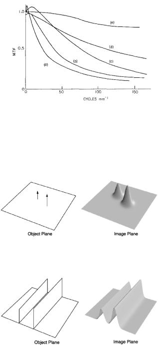
FIGURE 12.3. Some representative modulation transfer functions for various photographic films, showing how the resolution decreases as the film sensitivity increases. Film (a) has the greatest sensitivity and worst resolution. Film (e) is the least sensitive (“slowest”) and has the best resolution. With permission from R. Shaw. Photographic Detectors. Chapter 5 of Applied Optics and Engineering, New York, Academic, 1979. Vol. 7, pp. 121–154.
FIGURE 12.4. The point-spread function. Two impulse sources of di erent height are shown in the object plane. The response to them is shown in the image plane.
FIGURE 12.5. The line-spread function. Two line sources are shown in the object plane. The response to them is shown in the image plane.
12.2.3 Lineand Edge-Spread Functions
The line-spread function is the response of a system to a line object in a plane perpendicular to the axis of the lens. In general, the system is not isotropic and the linespread function depends on the orientation of the line. The Fourier transform of the line-spread function along the y axis is Ch(kx, 0) and Sh(kx, 0). Figure 12.4 shows a geometrical interpretation of the point-spread function.
12.3 Spatial Frequencies in an Image |
329 |
Figure 12.5 shows the line-spread function. The edgespread function is the response to an object that has a step in the radiance. All of these functions are interrelated. A discussion of how one can be obtained from another is found in many places, including Chapter 9 of Gaskill (1972).
12.3 Spatial Frequencies in an Image
There are some universal relationships between the spatial frequencies present in an image and the character of the image. These relationships hold whether the image is a photograph, an x-ray film, a computed tomographic scan, an ultrasound or nuclear medicine image, or a magnetic resonance image. In this section we describe these general relationships, which we will use throughout the rest of the book.
The first general relationship concerns the size of an image and the lowest spatial frequency present. For simplicity, consider the x direction and the corresponding spatial frequencies k. The object is nonperiodic. But its image is represented by a Fourier series which has period L. We saw in Chapter 11 that if the lowest angular frequency present is ω0, the period is T = 2π/ω0. The lowest spatial frequency present (other than zero) is k0 = 2π/L. The series has harmonics with separation ∆k = k0. This leads to the fundamental relationship
L = |
2π |
. |
(12.21) |
|
|||
|
k0 |
|
|
The lowest spatial frequency present (which equals the separation of the spatial frequencies) determines the size of the image L (the “field of view” or FOV).
The second general relationship concerns the spatial resolution in an image and the highest spatial frequency present. If the image has N discrete samples, then the sampling interval or spatial resolution is ∆x = L/N. This allows (or requires) the determination of N/2 cosine co- e cients and N/2 sine coe cients. The highest spatial frequency present is kmax = N ∆k/2. We obtain
∆x = |
L |
|
∆k |
= |
π |
. |
(12.22) |
|
|
|
|||||
|
2 kmax |
kmax |
|
||||
The spatial resolution is inversely proportional to the highest spatial frequency present. As we saw for the Fourier series representing a square wave, the higher harmonics give fine detail and sharpness to the image.
To reiterate: The lowest spatial frequency in the image determines the field of view. The lower the minimum spatial frequency, the larger the field of view. The highest spatial frequency in the image determines the resolution. The higher the maximum spatial frequency, the finer the resolution.
Here are a number of pictures that show how changing the coe cients in certain regions of k space a ect an
330 12. Images
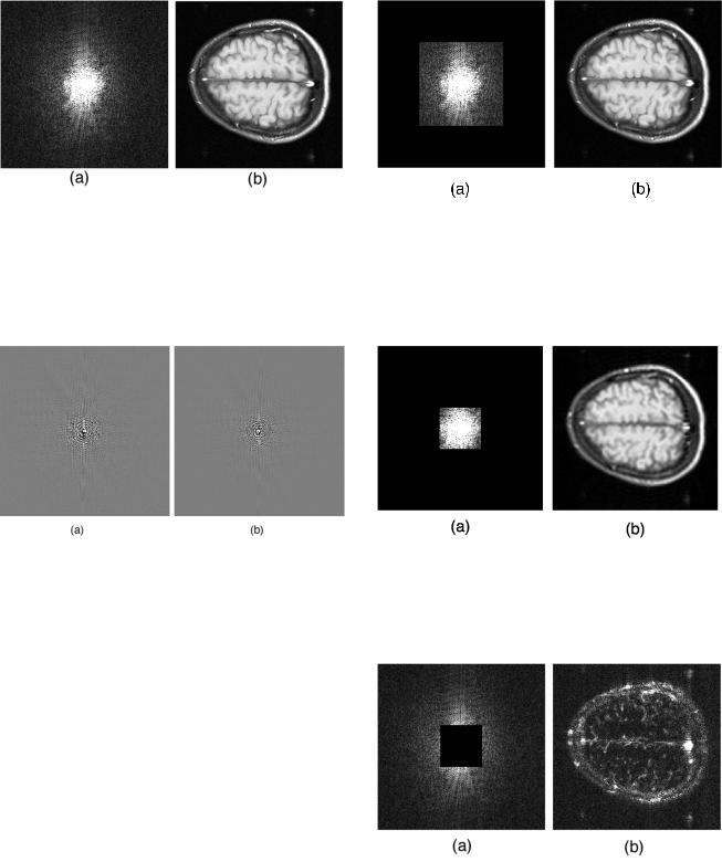
FIGURE 12.6. A magnetic resonance imaging head scan: (a) The squared amplitude C2 + S2 in k space. (b) The image. This is a normal image to compare with the following figures. Prepared by Mr. Tuong Huu Le, Center for Magnetic Resonance Research, University of Minnesota. Thanks also to Professor Xiaoping Hu.
FIGURE 12.7. The sine and cosine coe cients for the image in Fig. 12.6. (a) C(kx, ky ). (b) S(kx, ky ). Prepared by Mr. Tuong Huu Le, Center for Magnetic Resonance Research, University of Minnesota. Thanks also to Professor Xiaoping Hu.
image. Figure 12.6(b) shows a transverse scan of a head by magnetic resonance imaging. This is a normal image to compare with the following figures. It consists of 256 samples in each direction or 256 × 256 pixels. The magnitude of its Fourier transform is shown in Fig. 12.6(a). Figure 12.7 shows the cosine and sine coe cients in the expansion.
Figures 12.8 and 12.9 show what happens when the high-frequency Fourier components are removed. In the first case they have been removed above kx max/2 and ky max/2. In the second they are removed above kx max/4 and ky max/4. Compare the blurring in these figures with the original image.
When the low-frequency coe cients are set to zero as in Fig. 12.10, only the high-frequency edges remain. In this case the Fourier components below kx max/4 and ky max/4 have been set to zero. (Keeping the same values of kx max and ∆k and removing the information on those coe - cients keeps the field of view the same.)
FIGURE 12.8. The image that results when the high-fre- quency Fourier components above kx max/2 and ky max/2 are removed. Note the blurring compared to Fig. 12.6. Prepared by Mr. Tuong Huu Le, Center for Magnetic Resonance Research, University of Minnesota. Thanks also to Professor Xiaoping Hu.
FIGURE 12.9. The image that results when the high-fre- quency Fourier components above kx max/4 and ky max/4 are removed. The blurring is even greater. Prepared by Mr. Tuong Huu Le, Center for Magnetic Resonance Research, University of Minnesota. Thanks also to Professor Xiaoping Hu.
FIGURE 12.10. The image that results when the low-fre- quency Fourier components below kx max/4 and ky max/4 are removed. Prepared by Mr. Tuong Huu Le, Center for Magnetic Resonance Research, University of Minnesota. Thanks also to Professor Xiaoping Hu.
12.4 Two-Dimensional Image Reconstruction from Projections by Fourier Transform |
331 |
FIGURE 12.11. The Fourier coe cients for every other value of k have been set to zero. This has the e ect of doubling ∆k in Eq. 12.21. Since the width of the image has not been changed, this leads to aliasing, which shows up as the ghost images. (a) Every other value of kx has been removed. (b) Every other value of both kx and ky has been removed. Prepared by Mr. Tuong Huu Le, Center for Magnetic Resonance Research, University of Minnesota. Thanks also to Professor Xiaoping Hu.
Figure 12.11 shows the aliasing that results from setting every other Fourier coe cient to zero. This has the e ect of doubling ∆k in Eq. 12.21. Since the width of the image has not been changed, this leads to aliasing, which shows up as the “ghost” images. In the first case alternate Fourier coe cients have been removed in kx space; in the second they have been removed in both kx and ky .
12.3.1 Summary
In summary: The lowest spatial frequency in the image determines the field of view. The lower the minimum spatial frequency, the larger the field of view. Low spatial frequencies provide shape, contrast, and brightness.
The highest spatial frequency in the image determines the resolution. The higher the maximum spatial frequency, the finer the resolution. High spatial frequencies provide resolution, edges, and sharp detail.
12.4Two-Dimensional Image Reconstruction from Projections by Fourier Transform
The reconstruction problem can be stated as follows. A function f (x, y) exists in two dimensions. Measurements are made that give projections: the integrals of f (x, y) along various lines as a function of displacement perpendicular to each line. For example, integration parallel to the y axis gives a function of x,
∞
F (x) = |
f (x, y) dy, |
(12.23) |
−∞
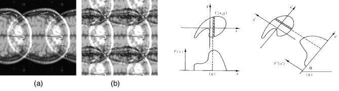
FIGURE 12.12. (a) Function F (x) is the integral of f (x, y) over all y. (b) The scan is repeated at angle with the x axis.
as shown in Fig. 12.12. The scan is repeated at many different angles θ with the x axis, giving a set of functions F (θ, x ), where x is the distance along the axis at angle θ with the x axis. The problem is to reconstruct f (x, y) from the set of functions F (θ, x ). Several di erent techniques can be used. A detailed reference is the book by Cho et al. (1993).
We will consider two of these techniques: reconstruction by Fourier transform, where the Fourier coe cients are obtained from projections (in this section), and filtered back projection (Sec. 12.5).
The Fourier transform technique is easiest to understand. Consider Eqs. 12.9. If ky = 0 in Eq. 12.9b, the result is
∞ |
|
∞ |
|
C(kx, 0) = |
cos(kxx)dx |
f (x, y)dy |
|
−∞ |
|
−∞ |
|
∞ |
|
|
|
= |
cos(kxx)F (θ = 0, x)dx. |
(12.24) |
|
−∞ |
|
|
|
Similarly |
|
|
|
∞ |
|
|
|
S(kx, 0) = |
sin(kxx)F (0, x)dx. |
(12.25) |
|
−∞ |
|
|
|
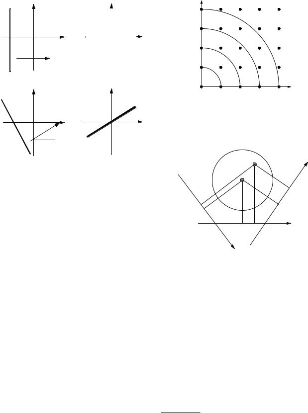
To state this in words: the Fourier transform of F (0, x) determines the sine and cosine transforms of f (x, y) along the line ky = 0 (the kx axis) in the spatial frequency plane. This is shown in Fig. 12.13.
A scan in another direction can be Fourier-transformed to give C and S at an angle θ with the kx axis. The Fourier transform of the projection at angle θ is equal to the two-dimensional Fourier transform of the object, evaluated in the direction θ in Fourier transform space. This result is known as the projection theorem or the central slice theorem (Problem 17). The transforms of a set of projections at many di erent angles provide values of C and S throughout the kxky plane that can be used in Eq. 12.9a to calculate f (x, y). In Chapter 18 we will find that the data from an MRI scan give the functions C(kx, ky ) and S(kx, ky ) directly.
In practice, the transforms are discrete. Using the notation that includes the redundant frequencies above N/2 and makes the coe cients half as large (Eqs. 11.27), the
332 12. Images
Integration
y |
|
|
ky |
|
m |
|
|
||||
|
|
|
|
|
|
|
|
C(kx ,0); S(kx ,0) |
|
|
|
|
|
|
|
|
|
x |
|
|
|
kx |
|
Scan |
|
|
|
|
|
|
|
|
|
|
|
y |
|
Integration |
|
Scan |
x |
|
|
θ |
|
ky |
θ |
kx |
FIGURE 12.13. The Fourier transform of F (θ = 0, x) =
f (x, y)dy gives Fourier coe cients C and S along the kx axis (ky = 0). The Fourier transform of scans at other angles θ give C and S along corresponding lines in the kxky plane.
two-dimensional discrete Fourier transform (DFT) is2
|
|
N −1 N −1 |
|
2π(jl + km) |
|
|||||||
fjk = Clm cos |
|
|
|
|
|
|
|
(12.26a) |
||||
|
|
N |
|
|
|
|
||||||
|
|
l=0 m=0 |
|
|
|
|
|
|
|
|||
|
|
|
|
|
|
|
|
|
|
|||
|
|
N −1 N −1 |
2π(jl + km) |
|
|
|
|
|||||
+ Slm sin |
|
|
|
. |
|
|||||||
|
|
N |
|
|||||||||
|
|
l=0 m=0 |
|
|
|
|
|
|
|
|||
|
|
|
|
|
|
|
|
|
|
|||
The coe cients are given by |
|
|
|
|
|
|
|
|
||||
1 |
|
N −1 N −1 |
|
|
2π(jl + km) |
|
||||||
Clm = |
|
|
|
|
|
|
|
|
|
|
|
|
|
|
|
fjk cos |
|
|
|
|
, |
(12.26b) |
|||
N 2 |
|
|
N |
|
|
|||||||
|
|
|
|
j=0 k=0 |
|
|
|
|
|
|
|
|
1 |
|
N −1 N −1 |
|
|
2π(jl + km) |
|
||||||
Slm = |
|
|
|
|
|
|
|
|
|
|
|
|
N 2 |
fjk sin |
|
N |
|
. |
(12.26c) |
||||||
|
|
|
|
j=0 k=0 |
|
|
|
|
|
|
|
|
Making a DFT of the projections gives values for C and S that lie on the circles in Fig. 12.14. But taking the inverse transform to calculate the reconstructed image requires values at the lattice points. They are obtained by interpolation. The details of how the interpolation is made are crucial when using the Fourier transform reconstruction technique.
l
FIGURE 12.14. The two-dimensional Fourier reconstruction requires values of C and S at the lattice points shown. The Fourier transforms of the projections F (θ, x) give the coe - cients along the circular arcs. Interpolation is necessary to do the reconstruction.
B
|
A |
Scan |
3 |
|
|
||
Scan |
|
|
|
1 |
|
|
|
Scan 2
FIGURE 12.15. The principle of back projection. Each point in the image is generated by summing all values of F (θ, x ) that projected through that point. For point A at the center of rotation, the appropriate value of x is the same at each angle. For other points such as B, the value of x is di erent at each angle.
12.5Reconstruction from Projections by Filtered Back Projection
Filtered back projection is more di cult to understand than the direct Fourier technique.3 It is easy to see that every point in the object contributes to some point in each projection. The converse is also true. In a back projection every point in each projection contributes to some point in the reconstructed image. This can be seen from Figure 12.15, which shows two points A and B and three projections. For point A, which is at the center of rotation, the
2In this notation the low frequencies occur for low values of the indices l and m. Usually, as in Figs. 12.6–12.11, the indices are shifted so k = 0 occurs in the middle of the sum.
3A simple experiment on back-projection using a laser pointer is described by Delaney and Rodriguez (2002).
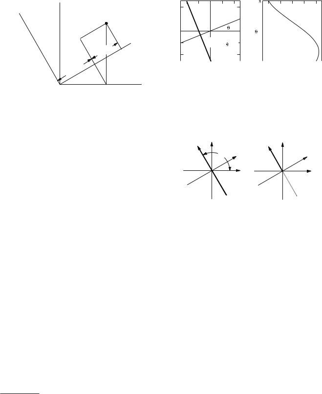
y
y'
P
θ ysin
θ |
θ |
|
cos |
||
|
||
x |
|
12.5 Reconstruction from Projections by Filtered Back Projection |
333 |
2
x0 = 2, y0 = 1 1 


x'
y 0
Path of integration
-1
to obtain F( ,x')
x'
-2
|
|
|
|
|
|
|
|
0 |
|
|
|
|
|
|
|
|
|
-2 |
-1 |
0 |
1 |
2 |
-2 |
-1 |
0 |
1 |
2 |
||||||||
|
|
|
|
x |
|
|
|
|
|
|
|
|
x' |
|
|
|
|
θ
x
FIGURE 12.16. By considering components of the coordinates of point P in both coordinate systems, one can derive the transformation equations, Eqs. 12.27 and 12.28.
(a) |
(b ) |
FIGURE 12.17. An object and its sinogram. The object is a δ function at (x0, y0). (a) The object and the path of a projection at angle θ. (b) A sinogram of the object F (θ, x ). The value of F would be plotted on an axis perpendicular to the x θ plane. The line shows the values of θ and x for which F is nonzero.
relevant value of x is the same in each projection, while for point B the value of x is di erent in each projection.
A very simple procedure would be to construct an image by back-projecting every projection. The back projection fb(x, y) at point (x, y) is the sum of F (θ, x ) for every projection or scan, using the value of x that corresponds to the original projection through that point. That is, for Fig. 12.15, the back projection at point A would be the sum of the three values for which the solid projection lines intersect the scans, while for point B it would be the sum of the values where the three dashed lines strike the scans. This gives a rather crude image, but we will see how to refine it.4
Figure 12.16 shows how to relate the values of x and y for a projection at angle θ to the object or image coordinates x and y. The transformations are
y ' |
θ ' |
|
(a) |
(b) |
FIGURE 12.18. Integration for the back projection is over y from −∞ to +∞,as shown in (a). This can be converted to an integral from 0 to ∞ if the angular integration is taken from 0 to 2π, as shown in (b).
x = x cos θ + y sin θ,
y = −x sin θ + y cos θ,
and the inverse transformations are
x = x cos θ − y sin θ,
y = x sin θ + y cos θ.
(12.27)
(12.28)
The process of calculating F (θ, x ) from f (x, y) is sometimes called the Radon transformation. When F (θ, x ) is plotted with x on the horizontal axis, θ on the vertical axis, and F as the brightness or height on a third perpendicular axis, the resulting picture is called a sinogram. For
example, the projection of f (x, y) = δ(x − x0)δ(y − y0) is F (θ, x ) = δ(x − (x0 cos θ + y0 sin θ)). A plot of this object and its sinogram is shown in Fig. 12.17.
The definition of the back-projection is
The projection at angle θ is integrated along the line y :
F (θ, x ) = f (x, y) dy
|
π |
|
fb(x, y) = |
F (θ, x ) dθ, |
(12.30) |
|
0 |
|
where x is determined for each projection by using Eq.
=f (x cos θ − y sin θ, x sin θ + y cos θ)dy . 12.27. The limits of integration are 0 and π since the
(12.29)
4To see why it is crude, suppose the original object is a disk at the origin. Every projection will be the same because of the symmetry in angle. Every back projection will lay down a contribution to the image along a stripe. Even though the reconstructed image will be largest where the original circle was, the image will have nonzero values throughout the image plane. We will see this example in Sec. 12.6.
projection for θ + π repeats the projection for angle θ. We will now show that the image fb(x, y) obtained by
taking projections of the object F (θ, x ) and then backprojecting them is equivalent to taking the convolution of the object with the function h(x−x , y −y ) = 1/r, where r is the distance in the xy plane from the object point to the image point. Function h depends only on the distance between the object and image points. This is discussed in greater detail by Barrett and Myers (2004, p. 280). To

334 12. Images
simplify the algebra, we find the back projection at the origin. We want the set of projections for x = 0 as a function of scan angle θ. They are, from Eq. 12.29,
∞
F (θ, 0) = |
f (−y sin θ, y cos θ) dy . |
(12.31) |
|
−∞ |
|
In terms of angle θ = θ + π/2 which is the angle from the x axis to the y axis,
∞
F (θ , 0) = f (y cos θ , y sin θ ) dy .
−∞
The arguments of f look very much like components of a vector, with magnitude r and components r cos θ and r sin θ . This suggests expressing the integral in polar coordinates. Since y is a dummy variable, call it r . In terms of r and θ the projection is
∞
F (θ , 0) = |
f (r , θ ) dr . |
(12.32) |
|
−∞ |
|
Inserting this expression in Eq. 12.30 gives for the back projection
|
π |
∞ π |
fb(0, 0) = |
F (θ , 0)dθ = |
f (r , θ ) dr dθ . |
|
0 |
−∞ 0 |
|
|
(12.33) |
Figure 12.18(a) shows how y (that is, r ) is integrated from −∞ to ∞ while θ goes from 0 to π. For the purposes of Eq. 12.33 the limits of integration can be changed as in Fig. 12.18(b). Variable r can range from 0 to ∞ while θ goes from 0 to 2π. Then the expression for fb looks even more like an integration in polar coordinates:
∞ 2π
fb(0, 0) = |
f (r , θ ) dr dθ . |
0 |
0 |
There is still one di erence between this and polar coordinates. The element of area, which is dx dy in Cartesian coordinates, is r dr dθ in polar coordinates. Therefore, let us rewrite this as
∞ 2π f (r , θ ) |
|
|
||
fb(0, 0) = |
|
r dr dθ . |
(12.34) |
|
r |
||||
0 0 |
|
|
||
We now change to the Cartesian variables x and y . The back-projected image at the origin is
fb(0, 0) = |
∞ ∞ |
f (x , y ) |
(12.35) |
|||
−∞ −∞ |
|
dx dy . |
||||
(x 2 + y 2)1/2 |
||||||
For an arbitrary point (x, y) the result is similar: |
||||||
fb(x, y) = |
∞ ∞ |
|
f (x , y ) |
dx dy . |
||
−∞ −∞ [(x − x )2 + (y − y )2]1/2 |
||||||
|
|
|
|
|
|
(12.36) |
We have shown that the image obtained by taking projections of the object F (θ, x ) and then back projecting them is equivalent to taking the convolution of the object with the function h(x − x , y − y ) = 1/r, where r is
the distance in the xy plane from the object point to the image point.
The back-projected image is not a faithful reproduction of the object. But it is possible to manipulate the projections F (θ, x ) to produce a function G(θ, x ) whose back projection is the desired f (x, y). This is the process of filtering before making the back projection. To find the relationship between F and the desired function G, note that there is some function g(x, y) that we do not know, but which, when projected and then back projected, yields the desired function f (x, y). That is,
f (x, y) = gb(x, y) = |
|
(12.37) |
|
∞ ∞ |
|
g(x , y ) |
dx dy . |
−∞ −∞ [(x − x )2 + (y − y )2]1/2 |
|||
Equations 12.10 relate the Fourier coe cients of f , g, and h(r) = 1/r:
Cf (kx, ky ) = Cg (kx, ky )Ch(kx, ky ) − Sg (kx, ky )Sh(kx, ky ), Sf (kx, ky ) = Cg (kx, ky )Sh(kx, ky ) + Sg (kx, ky )Ch(kx, ky ).
These can be solved for |
|
|
|
Sg = |
ChSf − ShCf |
, |
|
|
C2 |
+ S2 |
|
|
h |
h |
(12.38) |
|
|
|
|
Cg = |
ChCf + ShSf |
. |
|
|
|||
|
C2 |
+ S2 |
|
|
h |
h |
|
One can show by direct integration (see problem 28) that the Fourier transform of h(r) = 1/r is
Ch(kx, ky ) = 2π(kx2 + ky2)−1/2,
(12.39)
Sh(kx, ky ) = 0,
so that
Cg (kx, ky ) = 21π (kx2 + ky2)1/2Cf (kx, ky ),
(12.40)
Sg (kx, ky ) = 21π (kx2 + ky2)1/2Sf (kx, ky ).
If function g(x, y) were known and were projected to give G(θ, x ), then back-projecting G would give the desired f (x, y). The final step is to relate G(θ, x ) and F (θ, x ) so that we do not have to know g(x, y). To establish this relationship, consider a projection on the x axis. Equations 12.24 and 12.25 show that
1 ∞
2π −∞
[Cf (kx, 0) cos(kxx) + Sf (kx, 0) sin(kxx)] dkx,
1 ∞
2π −∞
[Cg (kx, 0) cos(kxx) + Sg (kx, 0) sin(kxx)] dkx.
Equations 12.40 relate the Fourier coe cients for F and G. For ky = 0, (kx2 + ky2)1/2 = |kx|. Therefore
G(0, x) =
1
2π −∞
+ Sf (kx, 0) sin(kxx)] |kx| dkx. (12.41)
This result is independent of the choice of axis, so it must be true for any projection. There is a function h(x) which can be convolved with any F (θ, x) to give the desired function G(θ, x). Equation 12.41 shows that
Cg (kx, 0) = Cf (kx, 0) |kx| /2π,
Sg (kx, 0) = Sf (kx, 0) |kx| /2π.
Comparison with Eqs. 12.9 shows that
Ch = |kx| /2π, |
Sh = 0. |
||
Therefore |
|
|
|
|
1 |
2 ∞ |
|kx| cos(kxx) dkx. |
h(x) = |
|
|
|
2π |
−∞ |
||
|
|
|
|
Because the integrand is an even function, we can multiply by 2 and integrate from zero to infinity. The integral to infinity does not exist. However, there is some maximum spatial frequency, roughly the reciprocal of the resolution we want, which we call kx max. We can therefore cut the integral o at this maximum spatial frequency and obtain
|
1 |
kx max |
|
|
|
|
|
|
|
|||||
h(x) = |
|
|
|
|
kx cos(kxx) dkx |
|
|
|||||||
2π2 |
0 |
|
|
|||||||||||
= |
1 |
|
cos(kxx) |
+ |
kx sin(kxx) |
kx max |
|
|||||||
|
2π2 |
|
|
|
x2 |
|
|
x |
0 |
|
||||
|
|
|
|
|
|
|
|
|
|
|
||||
= |
kx2 max |
|
2 sinc(ξ) |
− |
sinc2 |
(ξ/2) |
, |
(12.42) |
||||||
(2π)2 |
||||||||||||||
|
|
|
|
|
|
|
|
|||||||
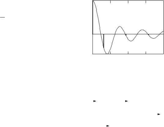
where ξ = kx maxx and sinc(ξ) = sin(ξ)/ξ. The function h(x) is plotted in Fig. 12.19. Using a sharp high-frequency cuto introduces some problems, which are described below and which are easily overcome.
To summarize: If each projection F is convolved with the function h of Eq. 12.42 and then back-projected, the back-projected image is equal to the desired image.
Figure 12.20 summarizes the two methods of reconstructing an image from projections.
12.6An Example of Filtered Back Projection
It is not di cult to write a computer program to perform filtered back projection if execution speed is not a concern. For our example we will use an object with circular symmetry, so that every projection is equivalent and only
12.6 An Example of Filtered Back Projection |
335 |
arbitrary units |
|
k = 1 |
k = 3 |
|
k = 5 |
), |
k = 0 |
|
|
|
|
h(ξ |
|
|
|
|
|
|
|
|
|
|
|
|
0 |
5 |
10 |
15 |
20 |
|
|
|
ξ |
|
|
FIGURE 12.19. The weighting function h(x) of Eq. 12.42. The bars show the nonzero values for the example in Section 12.6.
1-d Fourier |
|
|
Interpolate |
2-d inverse |
||||||
|
|
from polar |
||||||||
transform at |
|
|
to Cartesian |
Fourier |
||||||
each angle |
C( θ ,k) |
coordinates |
transform |
|||||||
C(kx ,ky ) |
||||||||||
F(θ,x') |
|
|
S( θ ,k) |
|
|
S(kx ,ky ) |
|
|
f(x,y) |
|
|
Convolve with |
|
|
|
|
|
||||
|
|
|
|
|
|
|||||
|
|
|
|
|
|
|
|
|||
|
|
function h(x) |
|
|
Back |
|
|
|||
|
|
at each angle |
G( θ ,x') |
project |
|
|
||||
|
|
|
|
|
|
|
|
|
||
|
|
|
|
|
|
|
|
|
||
FIGURE 12.20. A summary of the two methods for reconstructing an image.
one projection needs to be convolved with the weighting function h. Because of the circular symmetry the back projection is needed only along one diameter. The program shown in Fig. 12.21 was used to reconstruct the image.
The “top-hat” function is used as the object:
$ |
1, |
x2 + y2 < a2 |
(12.43) |
f (x, y) = |
0, |
otherwise. |
|
|
|
The projection is independent of θ: F (x) = 2(a2 − x2)1/2 for x2 < a2. Procedure CalcF evaluates F (x) for 100 points. Variables x and i are related by x = 2i/N − 1, so that x ranges from −1 to 1 as index i goes from 0 to 100. The value of a is 0.5.
The convolution is done by procedure Convolve, which uses convolving function h to operate on function F to produce G. The discrete form of h is obtained from Eq. 12.42 by the following argument, originally due to Ramachandran and Lakshminarayanan [see Cho et al., (1993), p. 80]. Variable x is considered on the interval (−1, 1), so the period is 2 and ω0 = π. The maximum spatial frequency is kx max = N π/2. The value of x in the weighting function h(x) depends on the value of index k = i − j: xi − xj = 2(i − j)/N = 2k/N . Therefore ξ = kx maxx = (N π/2)(2/N )k = πk, where k is an
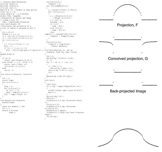
336 12. Images
FIGURE 12.21. The program used to make a filtered back projection of a circularly symmetric function.
integer. From Eq. 12.42 we obtain |
|
|||||
|
N 2/16, |
|
k = 0 |
|
||
|
|
|
|
|
|
|
h(k) = |
|
0, |
|
|
k even |
(12.44) |
|
2 |
2 |
π |
2 |
k odd. |
|
−N |
/4k |
|
|
|||
Procedure Convolve replaces the integral of Eq. 12.4a by a sum. The factor dx in the integral becomes 1/N in the sum.
Procedure BackProject forms the image from G. One hundred eighty projections are done in 1 ◦ increments from 0 to 179. The value of x is determined from x = i cos θ, but it is shifted so that the rotation takes place about i = 50. Unless x is at the end points, the value of G is obtained by linear interpolation. The value of ∆θ used to convert the integral to a sum is π/180.
Procedure PrintData writes the data for the plots shown in Fig. 12.22. One can see from inspection of Fig. 12.22 how the convolution converts the semicircular projection F into a function G that is flat-topped over the region of nonvanishing f and has a negative contribution in the wings. Figure 12.23 shows what the image looks
FIGURE 12.22. Reconstruction of a circularly symmetric image by filtered back projection. (a) The projection F (x). (b) The convolved projection G(x). (c) The image from back-pro- jecting the convolved data.
FIGURE 12.23. Reconstruction by simple back projection without convolution. The object is the same as in Fig. 12.22.
like if the back projection is done without first performing the convolution.
One can also see from Fig. 12.22 that ringing is introduced at the sharp edges. This is characteristic of the sharp high-frequency cuto at kx (similar to the Fourier series representation of a square wave with only a fi- nite number of terms). Early computer tomography (CT) scans created with the convolution function presented here showed a dark band just inside the skull where there was an abrupt change in f (x, y) upon going from bone to brain (Fig. 12.24). A gradual high-frequency cuto changes the details of h(k) and eliminates this ringing (Fig. 12.25).
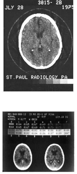
FIGURE 12.24. An early CT brain scan, showing ringing inside the skull. Photograph courtesy of St. Paul Radiology Associates, St. Paul, MN.
FIGURE 12.25. A set of brain scans using a gradual high-fre- quency cuto to eliminate ringing. Photograph courtesy of Professor J. T. Payne, Department of Diagnostic Radiology, University of Minnesota.
|
|
|
|
Symbols Used |
337 |
b |
Length of object |
m |
326 |
||
f, g |
Arbitrary functions |
|
326 |
||
fb, gb |
Back-projected images |
|
333 |
||
|
of f, g |
|
|
||
h |
Point-spread function; |
|
326 |
||
|
impulse response for |
|
|
||
|
convolution |
|
|
||
i |
√ |
|
|
|
327 |
−1 |
|
||||
j, k |
Subscript indices for |
|
332 |
||
|
data |
|
|
||
k, kx, ky |
Spatial frequencies |
m−1 |
326 |
||
l, m |
Subscript indices for |
|
332 |
||
|
Fourier coe cients |
|
|
||
m |
Magnification |
|
327 |
||
t, t |
Time or arbitrary vari- |
|
326 |
||
|
able |
|
|
||
x, y, x , y |
Distance; coordinates |
m |
327 |
||
|
in image or object |
|
|
||
|
plane; rotated |
|
|
||
|
coordinate system for |
|
|
||
|
image reconstruction |
|
|
||
A |
Amplitude |
|
326 |
||
Cf |
Fourier cosine |
|
326 |
||
|
transform of function |
|
|
||
|
f |
|
|
||
D |
Length of image |
m |
329 |
||
E |
Function describing an |
|
327 |
||
|
image |
|
|
||
F |
Projection of function |
|
331 |
||
|
f |
|
|
||
F, G, H |
Complex Fourier |
|
327 |
||
|
transforms of f, g, h |
|
|
||
L |
Property describing |
|
327 |
||
|
an object |
|
|
||
L |
Width of image or |
m |
329 |
||
|
field of view (FOV) |
|
|
||
N |
Total number of data |
|
329 |
||
|
points; number of |
|
|
||
|
discrete values in one |
|
|
||
|
dimension of an image |
|
|
||
Sf |
Fourier sine transform |
|
326 |
||
|
of function f |
|
|
||
T |
Period |
s |
326 |
||
δ |
Dirac delta function |
|
326 |
||
λ |
Wavelength |
m |
326 |
||
φ |
Phase |
|
326 |
||
θ, θ |
Angle |
|
331 |
||
τ1 |
Time constant |
s |
326 |
||
ω, ω0 |
Angular frequency |
(radian) s−1 |
326 |
||
ξ |
Dummy variable |
|
333 |
||
Symbols Used in Chapter 12
Symbol |
Use |
Units |
First |
|
|
|
used on |
|
|
|
page |
a, b |
Constants |
|
328 |
a |
Radius of “top-hat” |
m |
335 |
|
function |
|
|
Problems
Section 12.1
Problem 1 Compare Eq. 12.4a to Eqs. 4.73 and 7.21 and deduce the impulse response for those two systems.