Добавил:
Опубликованный материал нарушает ваши авторские права? Сообщите нам.
Вуз: Предмет: Файл:

Intermediate Physics for Medicine and Biology - Russell K. Hobbie & Bradley J. Roth

.pdf
Скачиваний:
93
Добавлен:
10.08.2013
Размер:
20.85 Mб
Скачать

338 12. Images

FIGURE 12.26. Anatomic features shown in Fig. 12.25

Problem 2 Except for the minus sign, Eq. 12.4a is the same integral that defines the cross-correlation function. There are some important di erences, however. Show that the convolution function is commutative—interchanging the order of variables gives the same result—but that the cross-correlation function is not.

Problem 3 (a) Use the convolution integral, Eq. 12.4a, to calculate the convolution g(t) of the function h(t−t )in Eq. 12.5 with

$

1, 0 < t < T, f (t) = 0, otherwise .

Plot f (t) and g(t).

(b) Calculate the Fourier transform of g(t), h(t − t ), and f (t) from part (a), and show that they obey Eq. 12.6a.

Problem 4 Fill in the details in the derivation of Eq. 12.6a.

Problem 5 Use the convolution integral to calculate g(x) from h(x − x ) = a/[a2 + (x − x )2] and f (x) =

cos(kx). Interpret this physically as a spatial frequency filter. Hint:

cos(ky)dy

=

π

e−kb,

−∞


y2

+ b2


b


sin(ky)dy

= 0.

−∞


y2

+ b2


Problem 6 If you are familiar with complex variables, use the definition of the Fourier transform in Eq. 12.11a to prove the convolution theorem, Eq. 12.11b.

Problem 7 What are the two-dimensional images whose Fourier transforms are shown?

(a)ky

C = δ (kx k0 )δ (ky )

S = 0

kx

(b)ky

S = δ (kx k0 )δ (ky )

C = 0

kx

(c) ky

C

S = 0

θ

kx

Problem 8 Calculate the

two-dimensional Fourier

transform of the function


f (x, y) = $ 1,

−a/2 < x < a/2, −b/2 < y < b/2,

0,


otherwise.

Plot f (x, y)vs. x and y and Cf (kx, ky )vs. kx and ky for a = 2b.

Problem 9 Calculate

the

two-dimensional

Fourier

transform of the function


f (x, y) = sech

x

sech


y

.


a


b


You may need the relationship


π


πv


sech(uz) cos(vz)dz =


sech


.


0

2u

2u


Problem 10 Calculate the


two-dimensional

Fourier

transform of the function


$

1,

#


< a,


x2 + y2


f (x, y) =

0,

#


> a.


x2 + y2


Hint: convert to polar coordinates in both the xy and kxky planes, and use the facts that

J0(u) =

1

2π cos(u cos v)dv,

2π


0

uJ0(u)du = J1(u),

where J0 and J1 are Bessel functions of order zero and order one. Bessel functions are tabulated and have known properties, similar to trigonometric functions. See Abramowitz and Stegun (1972), p. 360.

Section 12.2

Problem 11 Complete the verification of Eq. 12.13 suggested in the text.

Problem 12 Find the Fourier transform of the pointspread function for the ideal imaging system, Eq. 12.13.

Problem 13 Use Eq. 12.15 to show that the sum of the squares of the Fourier coe cients of the image is equal to the sum of the squares of the Fourier coe cients of the object times the square of the modulation transfer function, for a given set of spatial frequencies (kx,ky ).

Problem 14 Write the modulation of the image in terms of the variables in Eq. 12.19.

Problem 15 How does magnification m change the spatial frequencies in going from object to image? Since one is concerned about seeing detail in the object, resolution and spatial frequencies are usually converted to object coordinates in medical imaging, while they are left in terms of the detector coordinates in photography.

Section 12.3

Problem 16 This problem shows how increasing the detail in an image introduces high-frequency components. Find the continuous Fourier transform of the two functions


0,

x < 0,


f1(x) = 1, 0 < x < 1,


0,

x > 1


0,


x < 0,


, 0 < x < 1/3,

#

3/2


0,


1/3 < x < 2/3,

f2(x) =


#


2/3 < x < 1,

3/2,


0,


x > 1.


Plot a(kx) = C2(kx) + S2(kx) 1/2 for each function using a spreadsheet or plotting package, for the range −45 < kx < 45. Compare the features of each plot. Both functions have the same value of f 2(x)dx.

Section 12.4

Problem 17 Prove the central slice theorem analytically. Consider the cosine term of the two-dimensional Fourier transform C(kx, ky ) in Eq. 12.9b. Rotate to the primed coordinates given by Eq. 12.28. Note that the area element dxdy transforms to dx dy . Express C as a function of polar coordinates in k-space, kx = k cos θ and

Problems 339

ky = k sin θ. Show that

C(θ, k) = F (θ, x ) cos(kx )dx ,

−∞

S(θ, k) = F (θ, x ) sin(kx )dx .

−∞

Problem 18 Suppose that f (x, y) is independent of y. Find expressions for C(kx, ky ) and S(kx, ky ) and insert them in the expression for f (x, y) to verify that f (x, y) is recovered. You will need Eqs. 11.65.

Problem 19 Suppose that the object is a point at the origin, so that f (x, y) = δ(x)δ(y). Find the projection F (x) and the transform functions C(kx, 0) and S(kx, 0). Use these results to reconstruct the image using the Fourier technique.

Problem 20 Figure 12.14 shows that taking the Fourier transform of the projection F (θ, x ) gives the Fourier coefficients C(k, θ) at points along circular arcs in frequency space. In order the get these coe cients at equally spaced points in x and y, interpolation is necessary. One simple method is to use “bilinear” interpolation (Press et al., 1992). Suppose you know the Fourier coe cients at points ri = ir, θj = jθ, and you want to get the Fourier co- e cients at points xn = nx, ym = my. For a given xn, ym, convert to polar coordinates to get r and θ, then find the four known points that “surround” the desired point. The value of the coe cient is

C(xn, ym) =

1

[C(ri, θj )(ri+1

− r)(θj+1

− θ)

rθ

+C(ri+1, θj )(r − ri)(θj+1 − θ)

+C(ri, θj+1)(ri+1 − r)(θ − θj )

+C(ri+1, θj+1)(r − ri)(θ − θj )].

Suppose C(r, θ) = sin(r)/r, which is also called sinc(r). If C is known at points with r = 0.5 and θ = π/8, evaluate C at point x = 2, y = 3 using bilinear interpolation. Compare this result to the exact value of C = sinc((x2 +y2)1/2). Try this for other points (xn, ym).

Section 12.5

Problem 21 Derive Eqs. 12.27 and 12.28.

Problem 22 An object is described by the function f (x, y) = e(x2+y2)/b2 .

(a) Find the Fourier transform C(kx, ky ) and S(kx, ky ) directly from Eqs. 12.9 b and c.

(b)

Find

the

projection F (θ, x ) using Eq. 12.29.

Then

take

the

one-dimensional Fourier transform of

F (θ, x )using the equations


C(θ, k) =

F (θ, x ) cos kx dx


−∞


S(θ, k) =

F (θ, x ) sin kx dx .

−∞

340 12. Images

Use k = kx2 + ky2 1/2 to express C and S in terms of kx and ky . Your answer should be the same as part (a).

Use the following integral table:


az2

"

π


e

dz =


a


−∞


az2


"

π


b2/4a

e

cos bz dz =


e


−∞


a


e−az2

sin bz dz =

0.


−∞


Problem 23 Assume you have just measured the projection function F (θ, x ) = π1/2be(x −a cos θ)2/b2 . (For this problem, ignore the fact that your measuring device would only give F at discrete values of θ and x .) Find f (x, y). You may need the integrals from Problem 22.

Problem 24 Repeat Prob. 23 using


a


2 2

x 2


π

F (θ, x ) =


e−x /a

1 + cos2 θ

2


1 .

2


a2

Look up any integrals you need.

Problem 25 Suppose an object is a point at the origin, f (x, y) = δ(x)δ(y).The projection is also a point: F (θ, x ) = δ(x ). Calculate the back projection fb(x, y) (without filtering) using Eq. 12.30. To solve the problem, use this property of δ functions:

δ(g(u)) = δ(u − ui) , i |dg/du|u=ui

where the ui are the points such that g(ui) = 0. Note that the back projection is not a point. Back projection without filtering does not recover the object.

Problem 26 This problem is an extension of Prob. 25, but the object is no longer at the origin. Let f (x, y) =

δ(x − x0)δ(y − y0).

(a) Calculate F (θ, x ). You may need the following

properties of the δ function: δ(b−z)δ(z−a)dz = δ(b−a), δ(az) = δ(z)/|a|.

(b) Use the function F (θ, x ) you found in part (a) to calculate the back projection fb(x, y) using Eq. 12.30. You will need the property of the δ function given in Prob. 25.

(c) Show that fb(x, y)is equivalent to the convolution

#

of f (x, y)with the function 1/ (x − x )2 + (y − y )2.

Problem 27 Here is an easy way to show that the back projection fb(x, y)cannot be equivalent to the object

f (x, y). If f (x, y) is dimensionless, determine the units of F (θ, x ) and fb(x, y). Do f (x, y) and fb(x, y) have the same units?

Problem 28 Consider the Fourier transform of 1/r. The coe cients are given by

C(kx, ky ) =

∞ ∞

dx dy cos(kxx + ky y)

,


−∞ −∞

(x2

+ y2)1/2


S(kx, ky ) =

∞ ∞

dx dy sin(kxx + ky y)

.


−∞ −∞

(x2

+ y2)1/2


Transform to polar coordinates (x = r cos θ, y = r sin θ). Show from symmetry considerations of the angular integral that S = 0. Use the facts about the Bessel functions in Problem 10 and

J0(kr)dr = 1/k

0

to derive Eqs. 12.39. The function J0(x) is a Bessel function of order zero. It is tabulated and has known properties, similar to a trigonometric function. [See Abramowitz and Stegun (1972, p. 360).]

Problem 29 An object consists of three δ functions at


Draw the sinogram of

(0, 2), (


3, −1), and (3, −1).

the object.


Problem 30 Let f (x, y) = 1/[(x −a)2 + y2 + b2]. Calcu-

late F (θ, x ).


Problem 31 Let

f (x, y)

= x/(x2 + y2)2.

Calculate

F (θ, x ). Hint:


du


u


1


1 u


=


+


tan


.


(u

2

+ v

2

)

2

2v2 (u2

+ v2)


3

v


2 |v|


Problem 32 Consider

the

object


f (x, y)

=

#

a/ a2 − x2 − y2 for |x| < a, and 0 otherwise.

(a)Plot f (x, 0) vs. x.

(b)Calculate the projection F (θ, x ). Plot F (0, x ) vs.

x .

(c)Use the projection from part (b) to calculate the back projection fb(x, y). Plot fb(x, 0)vs. x.

(d)Compare the object and the back projection. Explain qualitatively how they di er.

Section 12.6

Problem 33 Verify that


$ 2


, |x| < a

F (θ, x) =

a2 − x2


0,

|x| > a

is the projection of the function in Eq. 12.43.

Problem 34 Verify Eqs. 12.44.

Problem 35 Modify the program of Fig. 12.21 and run it without the convolution.

Problem 36 Modify the program of Fig. 12.21 to reconstruct an annulus instead of a top-hat function.

References

Abramowitz, M. and I. A. Stegun. (1972). Handbook of Mathematical Functions with Formulas, Graphs and Mathematical Tables. Washington, DC, U.S. Government Printing O ce.


References

341

Barrett, H. H., and K. J. Myers (2004). Foundations of

Ramachandran, G. N., and A. V. Lakshminarayanan

Image Science. New York, Wiley-Interscience.

(1971). Three-dimensional reconstruction from radi-

Cho, Z.-h., J. P. Jones, and M. Singh (1993). Founda-

ographs and electron micrographs: Application of con-

tions of Medical Imaging. New York, Wiley.

volutions instead of Fourier transforms. Proc. Nat. Acad.

Delaney, C., and J. Rodriguez (2002). A simple medical

Sci. U.S. 68: 2236–2240.


physics experiment based on a laser pointer. Amer. J.

Shaw, R. (1979). Photographic detectors. Ch. 5 of Ap-

Phys. 70(10): 1068–1070.

plied Optics and Optical Engineering, New York, Acad-

Gaskill, J. D. (1972). Linear Systems, Fourier Trans-

emic, Vol. 7, pp. 121–154.


forms, and Optics. 3rd. ed. New York, Wiley.

Williams, C. S., and O. A. Becklund (1972). Optics:

Press, W. H., S. A. Teukolsky, W. T. Vetterling, and B.

A Short Course for Engineers and Scientists. New York,

P. Flannery (1992). Numerical Recipes in C: The Art of

Wiley.


Scientific Computing, 2nd ed., reprinted with corrections,


1995. New York, Cambridge University Press.


13
Sound and Ultrasound

Sound (or acoustics) plays two important roles in our

x

x + dx

study of physics in medicine and biology. First, ani-


mals hear sound and thereby sense what is happening in


their environment. Second, physicians use high-frequency


sound waves (ultrasound ) to image structures inside the


(a)

body. This chapter provides a brief introduction to the


physics of sound and the medical uses of ultrasonic imag-

ξ(x,t)

ξ (x + dx,t)

ing. A classic textbook by Morse and Ingard (1968) pro-


vides a more thorough coverage of theoretical acoustics,


and books such as Hendee and Ritenour (2002) describe

sn(x,t)

sn(x + dx,t)

the medical uses of ultrasound in more detail.


(b)

In Sec. 13.1 we derive the fundamental equation gov-


erning the propagation of sound: the wave equation. Sec-

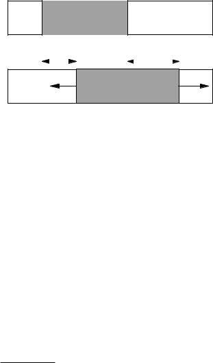
FIGURE 13.1. An elastic rod. (a) The rod in its equilibrium

tion 13.2 discusses some properties of the wave equation,

position. (b) Each point on the rod has been displaced from its

including the relationship between frequency, wavelength,

equilibrium position by an amount ξ which depends on x and

and the speed of sound. The acoustic impedance and

t. As a result there is a normal stress sn which also depends

its relevance to the reflection of sound waves are intro-

on x and t.


duced in Sec. 13.3. Section 13.4 describes the intensity


of a sound wave and develops the decibel intensity scale.

rium position. In this section we consider sound waves

The ear and hearing are described in Sec. 13.5. Section

propagating along the x axis. The results can be general-

13.6 discusses attenuation of sound waves. Physicians use

ized to three dimensions [See Morse and Ingard (1968)].

ultrasound imaging for medical diagnosis, as described in

We first consider an elastic rod, and then a fluid in which

Section 13.7. Ultrasonic imaging can provide information

viscous e ects are not important.

about the flow of blood in the body by using the Doppler


e ect, as shown in Sec. 13.8.

13.1.1 Plane Waves in an Elastic Rod


13.1

The Wave Equation

The simplest case to consider is an elastic rod which is

forced to move longitudinally at one end. This results in

In Chapter 1, we assumed that solids and liquids are in-

the propagation of a sound wave along the rod.1 We set up

a coordinate system where x measures distance along the

compressible. If a long rod were truly incompressible, a

rod from a fixed origin when no sound wave is traveling

displacement of one end would instantly result in an iden-

along the rod. We also assume that the disturbance of

tical displacement of the other end. In fact, the displace-

the rod depends only on the position along the rod, x,

ment does not propagate instantaneously. It travels at the


speed of sound in the rod.

1This simple geometry assures that all motion is parallel to the x

The propagation of sound involves small displacements

axis. In general, motion in an elastic solid involves both longitudinal

of each volume element of the medium from its equilib-

waves and transverse waves.


344 13. Sound and Ultrasound

and not on y or z, which are perpendicular to x. A wave in three dimensions that depends only on one dimension is called a plane wave.

When the sound travels along the rod, the material at point x is displaced from its undisturbed position by a small amount ξ(x, t), as shown in Fig. 13.1. The material originally at x + dx is displaced by amount ξ(x + dx, t). Since ξ(x + dx, t) is in general di erent from ξ(x, t), there is a strain in the rod (Eq. 1.24)

n(x, t) =

l

=

ξ(x + dx, t) − ξ(x, t)

=

∂ξ

. (13.1)

l

dx

∂x


Young’s modulus, E, relates the stress in the rod, sn, to the strain, n (Eq. 1.25):

sn(x, t) = E n(x, t) = E

.

(13.2)


dx


The di erence between the stress at each end, multiplied by the cross-sectional area of the rod, S, provides a net force that accelerates the shaded volume element in Fig. 13.1. The net force on the volume element is

Fnet = S [sn(x + dx, t) − sn(x, t)] = S ∂s∂xn dx = SE ∂xn dx.

Fnet = SE

2

ξ

dx.

(13.3)


∂x2


The mass of the shaded volume is ρSdx, where ρ is the density, and the acceleration of the volume is 2ξ/∂t2. [Since we are not subtracting a value at one end from the value at the other, and since we are taking the limit as dx → 0, we can ignore changes in ξ in the interval (x, x + dx).] Therefore, Newton’s second law becomes

2ξ

=

ρ ∂2ξ

.

(13.4)


∂x2

E ∂t2


This is the wave equation, and it is seen in many contexts, from the vibrations of a string to the propagation of electromagnetic waves. It is usually written as

2ξ

=

1 2ξ

,

(13.5)

2

c

2


∂t

2

∂x


where c is the speed of propagation of sound in the rod. In this case


*


c =

E

.

(13.6)


ρ


As Young’s modulus becomes very large or the density of the rod becomes very small, the speed with which a disturbance travels from one end of the rod to the other becomes larger and larger.


x

x + dx


SP0


SP0


(a)


ξ

(x,t)


ξ(x + dx,t)


SP(x,t)


SP(x + dx,t)


(b)

FIGURE 13.2. Sound propagates in one dimension in a fluid in a tube of cross-sectional area S. (a) In equilibriuim the pressure is p0 and the force on the shaded volume of fluid has magnitude p0S on each end. (b) When the sound is propagating, the forces on each end are as shown.

e ects. Changes in the fluid caused by the sound wave depend only on x and t.2 To make it easier to imagine the situation, suppose the fluid is confined in a tube. Then we can construct a figure very similar to Fig. 13.1. A small volume of fluid at rest extends from position x to x + dx, with cross-sectional area S as shown in Fig. 13.2(a). The force pushing on the left side of the volume is SP0, and the force on the right is −SP0.3 Here P0 is the pressure when the fluid is undisturbed by a sound wave. In equilibrium there is no net force on the volume element.

When the fluid element is displaced, as in Fig. 13.2(b), the net force to the right on the fluid element is


∂P

Fnet = S [P (x, t) − P (x + dx, t)] = −S


dx. (13.7)

∂x

The change of pressure from the equilibrium value P0 is related to the change of volume of the fluid by the compressibility, κ (Eq. 1.33):

P − P0 = p =

1 dV

=

1

,

(13.8)


κ V0

κ dx

from which


S ∂2ξ


Fnet =


dx.


(13.9)

κ ∂x2


To obtain the mass we use the volume Sdx times the equilibrium density ρ0. We multiply by the acceleration

of the fluid element, 2

ξ/∂t2, to obtain


2

ξ

= ρ0

κ

2ξ

.

(13.10)

∂x2

∂t2


13.1.2 Plane Waves in a Fluid

Now we consider a sound wave propagating in a fluid, where shear can be neglected. We also neglect viscous

2We might be looking at a wave whose properties depend on all three coordinates, x, y, and z, but where, in the region we are studying, the dependence on y and z is very slight. This is like the one-dimensional electrostatic approximations in Chapter 6.

3See Sec. 1.11; we ignore any forces arising from viscosity, gravity, or surface tension.

This is the wave equation, Eq. 13.5, with

c = "

1


.

(13.11)


κρ0


In both of these cases, the wave equation has been written in terms of the displacement of elements of the rod or the fluid from their equilibrium positions. It is also possible to show that the pressure, fluid density, and velocity of the fluid element also satisfy the wave equation. The pressure is discussed in Problem 2. The velocity of the fluid due to the sound wave is

v =

.

(13.12)


dt


Another important relationship is obtained by combining Eq. 13.12 with Eq. 13.8 and interchanging the order of di erentiation (Appendix N):

∂v

= −κ

∂p

(13.13)


.

∂x

∂t

Equations 13.8 and 13.10 can also be used to show that

∂v

=

1 ∂p

(13.14)


.

∂t

ρ0

∂x

Finally, since the density is ρ = M/V , we can show that


= κdp.

(13.15)


ρ0


In this section we have considered Young’s modulus E and compressibility κ. Remember from Chapter 3 that we can compress a gas at a constant temperature, and we can also do it adiabatically, when there is no heat flow and the temperature rises as the gas is compressed. The compressibility is di erent in these two cases. When static measurements of these parameters are made, there is usually time for the system being studied to remain isothermal. The pressure changes in a sound wave usually occur so rapidly that there is not time for heat to flow, and the adiabatic compressibility must be used. Values of Young’s modulus are also di erent for isothermal and adiabatic stresses and strains.

13.2 Properties of the Wave Equation

The parameter c in the wave equation has units of speed. To appreciate its physical interpretation, consider the departure from the undisturbed pressure p(x, t) = P (x, t) − P0 = f (x − ct), where f is any function. This solution obeys the wave equation (see Prob. 5). It is called a traveling wave. A point on f (x−ct), for instance its maximum value, corresponds to a particular value of the argument x − ct. To travel with the maximum value of f (x − ct), as t increases x must also increase in such a way as to keep x − ct constant. This means that the pressure distribution propagates to the right with speed c, as shown

13.2 Properties of the Wave Equation

345

f(x - ct)

t

x

FIGURE 13.3. A wave f (x−ct) travels to the right with speed c.

in Fig. 13.3. Solutions p(x, t) = g(x + ct), where g is any function, also are solutions to the wave equation, corresponding to a wave propagating to the left

The wave speed c is one of the most important parameters governing the propagation of sound waves. The density of water is about ρ0 = 1, 000 kg m3, and the compressibility of water is approximately 5×10¹⁰ Pa1, so the speed of sound in water is about 1,400 m s1. The speed of sound in tissue is similar but slightly higher; 1,540 m s1 is often taken as an average speed of sound in soft tissue. The speed of sound in air is about 344 m s1. See Denny (1993) for a more detailed comparison of

the speed of sound in air and water.


One

very

useful

traveling

wave

is

p(x, t) =

p0 sin

2π

(x

ct)

=

p0 sin 2π( x


t

)

=

p0 sin(kx


λ


λ

T


ωt). The pressure distribution oscillates sinusoidally with

frequency


f = c/λ

(13.16)

cycles per second (Hz) or angular frequency ω = 2πf (radians) s1. Equation 13.16 relates the frequency and wavelength. For instance, middle C has a frequency of 261.63 Hz. In air, the wavelength is (344 m s1)/(261.63 Hz) = 1.315 m. The wave number is

k =

2π

=

ω

.

(13.17)

λ


c


Standing waves such as

p(x, t) = p cos(ωt) sin(kx)

(13.18)

are also solutions to the wave equation. An example is shown in Fig. 13.4. The standing wave in Eq. 13.18 has nodes fixed in space where sin(kx) is zero. Standing waves can occur, for example, in an organ pipe and in the ear canal (Problem 7).

A standing wave can also be written as the sum of two sinusoidal traveling waves, one to the left and one to the right. Conversely, two standing waves can be combined to give a traveling wave (Problem 8).

346 13. Sound and Ultrasound

FIGURE 13.4. A standing wave f (x, t) = sin πx cos πt, plotted for 0 < x < 2 and 0 < t < 4.

Since the fluid velocity v obeys the wave equation, it can also be represented as a sinusoidal wave. It is important to realize that the fluid oscillates back and forth. The fluid itself does not propagate with the wave. What propagates is the disturbance in the fluid. Sound in a fluid is a longitudinal wave, which means that the fluid oscillates along the same axis that the disturbance propagates (in this case, both move in the x direction). Other types of waves exist in nature, such as electromagnetic waves studied in Chapter 14. Electromagnetic waves are transverse waves, because the electric field oscillates in a direction perpendicular to the direction of wave propagation. Solids, such as bones, can support shear stresses and can propagate both longitudinal and transverse acoustic waves. But fluids and soft tissue cannot support significant shear stresses and only propagate longitudinal waves.

pi(x)

Incident

pr(x)

Reflected

pt(x)

Transmitted

FIGURE 13.5. A sound wave with pressure amplitude pi traveling to the right is incident on a boundary separating tissue 1 on the left from tissue 2 on the right. Each tissue has a di erent density ρ0 and compressibility κ. Part of the wave is transmitted to the right with amplitude pt, and part is reflected to the left with amplitude pr . The drawing shows one instant in time when Z2 = 2Z1.

and the amplitudes are related by


κ

κλ


κc


ξ0 = p0


= p0


= p0


,

(13.22)

k

2π

ω

v0 =

p0


=

p0

.


(13.23)


ρ0c


Z


#

The quantity Z = ρ0c = ρ0is called the acoustic impedance of the medium.4 The acoustic impedance of water is about (103 kg m3)(1, 400 m s1) = 1.4 × 10⁶ Pa s m1. The acoustic impedance of air is about 400 Pa s m1, so Zair Zwater (Denny, 1993).

13.3 Acoustic Impedance

13.3.1Relationships Between Pressure, Displacement and Velocity in a Plane Wave

For a plane wave traveling to the right, the pressure, displacement and speed of the fluid have simple relationships. If the pressure change is

p(x, t) = p0 sin(kx − ωt),

(13.19)

one can use Eqs. 13.8 and 13.12 to show that the fluid displacement is

ξ = ξ0 cos(kx − ωt),

(13.20)

the fluid velocity is

v = v0 sin(kx − ωt),

(13.21)

13.3.2Reflection and Transmission of Sound at a Boundary

Consider next what happens at the boundary between two di erent media. Suppose a traveling wave is propagating to the right in a fluid with sound speed c1 and acoustic impedance Z1. At x = 0, it encounters a second fluid, with speed c2 and impedance Z2. In general, the interaction of the incoming wave with the boundary between the first and second fluids results in a reflected

4Strictly speaking, the acoustic impedance is the ratio Z = p0/v0, and carries information about both the amplitude ratio and the relative phase of the pressure and velocity. If the waves are in phase, Z is said to be “resistive;” if they are π/2 out of phase, Z is said to be “reactive.” The characteristic acoustic impedance is a property of the medium: Z0 = ρ0c. Both have units Pa m s1 or kg m2s1. For a plane wave the impedance is resistive and Z = Z0. For other waves, such as standing waves, there is a reactive component.

wave traveling to the left in fluid 1 and a transmitted (or refracted) wave traveling to the right in fluid 2 (Fig. 13.5). The acoustic impedances determine how much of the incoming wave is reflected and how much is transmitted. The waves must oscillate with the same frequency in both media. The pressure at the boundary must be the same in each medium, and the fluid velocity must also be continuous across the boundary. Let pi(x, t) =


ω


ω


pi sin


(x − c1t) , pr (x, t) = pr sin


(x + c1t) , and

c1

c1

pt(x, t) = pt sin

ω

(x − c2t) be the incoming, reflected,

c2

and transmitted pressures. The velocities are related to the pressures by the acoustic impedances. At the boundary, the pressure and the velocity must be continuous. In fluid 1 the amplitude of the pressure is pi + pr , and in fluid 2 it is pt. In fluid 1 the amplitude of the velocity is (pi − pr )/Z1, and in fluid 2 it is pt/Z2. (The minus sign arises because the reflected wave is traveling to the left.) Therefore

pi + pr = pt

(13.24)

and


(pi − pr )/Z1 = pt/Z2.

(13.25)

We can solve these two equations for pr and pt in terms of pi :

pr =

Z2

− Z1

pi,

(13.26)

Z2


+ Z1


pt =

2Z2

(13.27)


pi.

Z2 + Z1

The intensity I of a sound wave is a measure of the power per unit area (W m2). The instantaneous power per unit area transmitted by the wave in Eq. 13.19 at some point is

I(t) = p(t)v(t) = p0v0 sin2 ωt.

(13.28)

The average power per unit area is

I =

1


=

1 p2

(13.29)


p0v0


0

.

2


2 Z


Problems 13–15 show that the reflection and transmission coe cients are

R =

Ir


=


Z2

− Z1

2

,

(13.30)

Ii


Z2

+ Z1


and

It


4Z1Z2


T =

=


,


(13.31)


Ii


(Z1

+ Z2)2


and that R + T = 1.

If the acoustic impedance of the two fluids is the same, Z1 = Z2, there is no reflected wave and the entire incoming wave is transmitted. If Z1 Z2 (for example, sound going from air to water), almost all of the sound is reflected.

13.4 Comparing Intensities: Decibels

347

13.4 Comparing Intensities: Decibels

13.4.1The Decibel

When comparing two intensities, the range of di erences is often so great that a logarithmic comparison scale is used. We first saw the decibel when discussing the frequency response of a linear system in Chapter 11. Intensity levels in decibels (dB) have meaning only in terms of ratios:

I2

Intensity di erence (dB) = 10 log10 . (13.32)

I1

The intensity di erence can also be written in terms of pressure (or displacement or velocity) ratios:

Intensity di erence (dB)

= 10 log10

I2


= 10 log10

p2

2


I1


p1


= 20 log10

p2

.

(13.33)

p1


This assumes that p1 and p2 are measured in the same medium, so the acoustic impedance does not change. If the intensity of a wave falls to 1% of its original value, the intensity di erence is 10 log10(0.01) = 20 dB.

13.4.2 Hearing Response

In auditory acoustics, intensities are measured with respect to a reference intensity I0 = 1012 W m2. This is the intensity of the faintest sound that a person can typically hear:

Intensity level = 10 log10

I


(13.34)


.


I0


A sound that is 10 times as intense as the threshold for hearing has an intensity level of 10 dB. A sound with an average intensity I = 1 W m2 is perceived as painful, so the threshold for pain has an intensity level of about 120 dB. Table 13.1 gives the intensity in decibels for some common sounds.

The sensitivity of the ear depends on frequency. A typical hearing response curve for a young person is shown in Fig. 13.6. The minimum auditory field (MAF) is measured with a loudspeaker; the slightly di erent minimum auditory pressure (MAP) is measured with headphones. The ear is most sensitive to sounds between about 100 and 5,000 Hz. A sound at 20 Hz will not be perceived to be as loud as one at 1,000 Hz with the same intensity. Commercial sound level meters typically have two “weightings.” The “C” weighting has almost the same sensitivity at all frequencies. The “A” weighting more nearly mimics the response of the normal ear. Sounds with the same level when the meter is on “A” weighting will. be perceived as having the same loudness.

348 13. Sound and Ultrasound


10-4


80

-2

10-5


-6


m

10


60

W


10-7


Intensity,


10-8


40 dB

10-9


Sound

10-10


20

-11


10


10-12


0


10-13

102

103

104


101

Frequency, Hz

FIGURE 13.6. Hearing response (MAF) curve for a young adult.

FIGURE 13.7. A cross section of the ear. From J. R. Cameron, J. G. Skofronick, and R. M. Grant. Physics of the Body. Madison, WI. Medical Physics Publishing. 1999. Used by permission.

13.5 The Ear and Hearing

A cross section of the ear is shown in Fig. 13.7. The ear can be thought of as having three di erent sections, each with a unique purpose: the external ear gathers sound, the middle ear transfers energy from the air (low acoustic impedance) to the liquid of the inner ear (high acoustic impedance); the inner ear transforms the signal into nerve impulses going to the brain.

The external ear consists of the pinna, the visible part of the ear, and an air-filled tube called the ear canal.

The middle ear is a small chamber filled with air that contains three small bones, or ossicles (Fig. 13.8). It is separated from the ear canal by the ear drum. The bone in contact with the ear drum is called the malleus (it is shaped a bit like a mallet or hammer). The next bone is the incus (from the Latin for anvil, which it resembles slightly). The third bone, in contact with the oval window to the inner ear, is the stapes (again from the Latin, for stirrup.) The eustachian tube leads from the middle

TABLE 13.1. Approximate intensity levels of various sounds.

Sound

Intensity

Level (dB,


(W m2)

A weight-


ing)


Rocket launch pad

105

170


104

160


103

150

F-84 jet at takeo , 25 m

102

140

10

130

from the tail; Large


pneumatic riveting


machine (1 m); boiler


shop (maximum level);


peak sound level at a rock


concert


Sound that produces pain

1

120

Woodworking shop

101

110

Near a pneumatic drill

102

100

(“jack hammer”)


90

Inside a motor bus

103

Urban dwelling near

104

80

heavy tra c


70

Busy street

105

Speech at 1 meter

106

60

O ce

107

50

Average dwelling

108

40

Maximum background

109

30

sound level tolerable in a


broadcast studio


20

Whisper; maximum

1010

background sound level


tolerable in a motion


picture studio

1011

10


Minimum perceptible

1012

0

sound


ear to the mouth and throat (nasopharynx ). Since the ear is sensitive to very small pressure changes, the eustachian tube serves the important function of keeping the pressure on both sides of the ear drum the same for slow changes, such as when we climb stairs or the weather changes. The walls of the eustachian tube are often collapsed together. Swallowing helps to open them up and equalize the pressure if necessary.

Sound arrives at the ear as a vibration in air. Sound energy must enter the inner ear in order to be converted into a nerve signal to the brain. Yet, the inner ear is filled with liquid. The acoustic impedance of the liquid in the inner ear is about 3, 500 times larger than the acoustic impedance of air. This means that without the impedance transformation by middle ear, the intensity in the inner ear would be only about 1/1, 000 of the pressure amplitude in air—a loss of about 30 dB (Problem 14).