Intermediate Physics for Medicine and Biology - Russell K. Hobbie & Bradley J. Roth
.pdf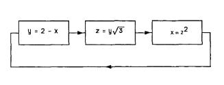
Problem 6 A feedback loop has the three stages shown. |
Suppose that exogenous phosphate is entering the plasma |
|||||||||||||||||
Find the operating point and the open-loop gain if these |
at a fixed rate R and that steady state has been reached |
|||||||||||||||||
variables are all positive. |
|
|
|
|
|
|
|
|
so that R = (dQ/dt)excreted into urine. |
|
|
|||||||
|
|
|
|
|
|
|
|
|
|
|
|
|
|
(a) What value for reabsorption does this imply? |
||||
|
|
|
|
|
|
|
|
|
|
|
|
|
|
(b) Determine two equations relating K and Cp and |
||||
|
|
|
|
|
|
|
|
|
|
|
|
|
|
plot them. |
|
|
||
|
|
|
|
|
|
|
|
|
|
|
|
|
|
(c) Calculate the open-loop gain of the feedback loop. |
||||
|
|
|
|
|
|
|
|
|
|
|
|
|
|
Problem 10 With considerable simplification, consider |
||||
|
|
|
|
|
|
|
|
|
|
|
|
|
|
the body to have a constant temperature T throughout and |
||||
|
|
|
|
|
|
|
|
|
|
|
|
|
|
a total heat capacity C. The total amount of thermal en- |
||||
Problem 7 Consider how thyroid hormone is removed |
ergy in the body is U . The heat capacity is defined so that |
|||||||||||||||||
from the body by the kidneys. The variables are V , the |
dU = CdT . The source of the thermal energy is the body’s |
|||||||||||||||||
total plasma volume (l); C, the plasma concentration of |
metabolism: (dU/dt)in = M . If sweating is ignored, the |
|||||||||||||||||
thyroid hormone (mol l−1); y, the total amount of hor- |
rate of loss of energy by convection and radiation is ap- |
|||||||||||||||||
mone (mol); and R, the rate of hormone production (mol |
proximately proportional to the amount by which the body |
|||||||||||||||||
s−1). In the steady state, the rate of change is dy/dt = |
temperature exceeds the ambient or surrounding temper- |
|||||||||||||||||
R − KC = 0. Then R = KC and y is not changing with |
ature: (dU/dt)loss = K(T − Ta). |
|
|
|||||||||||||||
time (see Chapter 2). The clearance K is a measure of |
(a) What is the steady-state temperature as a function |
|||||||||||||||||
the kidneys’ ability to remove hormone, since the removal |
of M and Ta? |
|
|
|||||||||||||||
process depends on the concentration. |
|
|
|
|
|
(b) Write a di erential equation for T as a function of |
||||||||||||
|
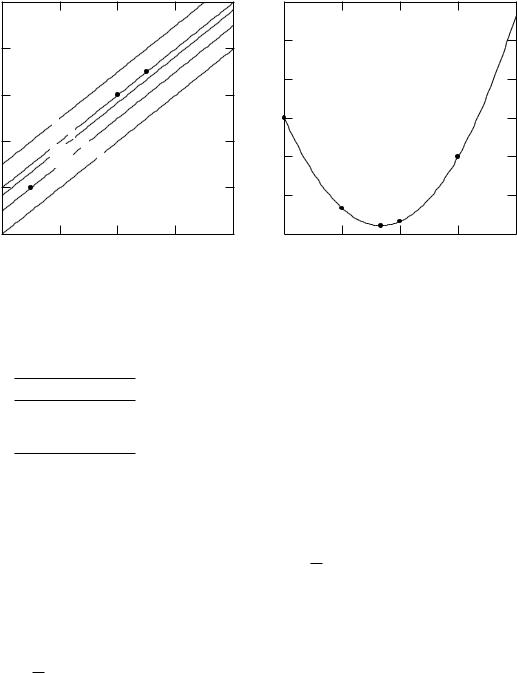
(a) Plot K vs C for two di erent values of R. Show on |
time. Suppose that M suddenly jumps by a fixed amount. |
||||||||||||||||
your graph what happens if K remains fixed as R changes. |
What is the time constant? |
|
|
|||||||||||||||
|
(b) It has been found experimentally [D. S. Riggs |
|
|
|
|
|||||||||||||
(1952). Pharmacol. Rev. 4: 284–370] that K increases |
Problem 11 When the body temperature is above 37 ◦C, |
|||||||||||||||||
as C increases: K = aC. Plot this on your graph, too. |
||||||||||||||||||
|
(c) Draw a block diagram showing the proper cause and |
sweating becomes important. The rate of energy loss is |
||||||||||||||||
e ect relationship between C and K. |
|
|
|
|
|
proportional to the amount of water evaporated. If all |
||||||||||||
|
(d) Calculate the open-loop gain. Show how changes in |
the perspiration evaporates, sweating loss can be approx- |
||||||||||||||||
C are altered by the feedback mechanism. |
|
|
|
|
|
imated by (dU/dt)sweat = L(T − 37). |
|
|
||||||||||
Problem 8 A substance is produced in the body and re- |
(a) Modify the di erential equation of the previous |
|||||||||||||||||
problem to include (dU/dt)sweat as the input variable with |
||||||||||||||||||
moved at rate R. The concentration is C. The clearance is |
T as the output variable. Combine it with this new equa- |
|||||||||||||||||
defined to be K. In the steady state 0 = dy/dt = R −KC, |
tion to make a feedback loop. Determine the new equilib- |
|||||||||||||||||
or K = R/C. It is found experimentally that the clear- |
rium temperature and the time constant. |
|
|
|||||||||||||||
ance depends on the concentration as K = aCn, where |
(b) Make numerical comparisons for the previous prob- |
|||||||||||||||||
C is the independent variable. Find the open-loop gain, |
lem and this one when M = 71 kcal h−1, C = 70 kcal |
|||||||||||||||||
eliminating K and a from your answer. |
|
|
|
|
|
◦C−1, K = 25 kcal h−1 ◦C−1, L = 750 kcal h−1 ◦C−1, |
||||||||||||
Problem 9 The kidney excretes phosphate in the follow- |
Ta = 38 ◦C (high enough to ensure sweating). |
|||||||||||||||||
|
|
|
|
|||||||||||||||
ing way. The total plasma volume Vp contains phosphate |
|
|
|
|
||||||||||||||
at concentration Cp: Qp = CpVp. A volume of plasma |
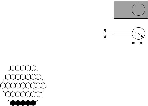
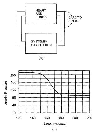
Problem 12 A simplified model of the |
circulation is |
||||||||||||||||
(dV /dt)f is filtered through the renal glomeruli into the |
||||||||||||||||||
shown. Normally we know that the arterial pressure is |
||||||||||||||||||
nephrons each second. Within the nephron, phosphate is |
||||||||||||||||||
the same as that in the carotid sinus: part = psinus. In |
||||||||||||||||||
either |
reabsorbed into the |
|
plasma or excreted |
into the |
||||||||||||||
|
experiments on dogs whose vagus nerves were cut, the |
|||||||||||||||||
urine. Experiments show that virtually all phosphate is |
||||||||||||||||||
carotid arteries were isolated and perfused by a separate |
||||||||||||||||||
reabsorbed up to some rate (dQ/dt)max: |
|
|
|
|
|
|||||||||||||
|
|
|
|
|
pump. This broke the feedback loop and allowed the curve |
|||||||||||||
|
|
|
|
|
|
|
|
|
|
|
|
|
|
|||||
|
|
|
|
Cp (dV /dt) |
f |
, |
Cp (dV /dt) |
f |
< (dQ/dt) |
max |
on the accompanying graph to be obtained. The empiri- |
|||||||
dQ |
= |
|
|
|
|
|
cal equation shown [based on the work of A. M. Scher and |
|||||||||||
|
dt |
reabs |
(dQ/dt)max , |
Cp (dV /dt)f ≥ (dQ/dt)max . |
A. C. Young, (1963). Serroanalysis of carotid sinus reflex |
|||||||||||||
|
|
|
|
|
|
|
|
|
|
|
|
|
e ects on peripheral resistance. Circ. Res. 12: 152–165, |
|||||
|
|
|
|
|
|
|
|
|
|
|
|
|
|
|||||
|
As in Problem 7(a), at equilibrium the clearance of |
summarized in Riggs (1970)] is (with pressures in torr) |
||||||||||||||||
|
|
|
|
|
||||||||||||||
phosphate from the plasma is defined as |
|
|
|
|
|
|
|
|
|
|||||||||
|
|
|
|
(dQ/dt)excreted into urine |
|
|
|
120 |
|
|
||||||||
|
|
|
|
|
|
|
part = 90 + |
|
|
. |
||||||||
|
|
|
|
|
|
|
|
|
||||||||||
|
|
|
K = |
|
|
|
|
|
|
. |
|
|
|
1 + exp [(psinus − 165)/5] |
||||
|
|
|
|
|
|
Cp |
|
|
|
|
|
|||||||
|
|
|
|
|
|
|
|
|
|
|
|
|
|
|||||
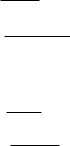
 APD
APD 
 DI
DI