Intermediate Physics for Medicine and Biology - Russell K. Hobbie & Bradley J. Roth
.pdf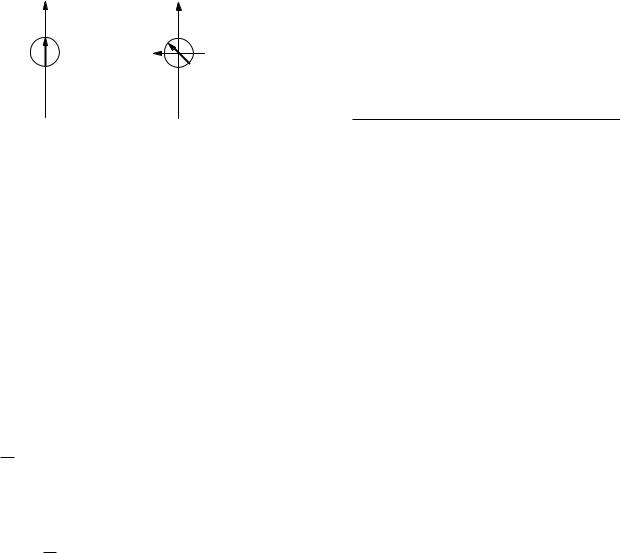
|
|
|
|
|
|
|
|
|
|
Problems |
249 |
||
Symbol |
Use |
Units |
First |
0 |
|
|
Electrical permittivity |
C2 |
N−1 |
229 |
|||
|
|
|
used on |
|
|
|
of vacuum |
|
|
m−2 |
|
||
|
|
|
page |
κ |
|
|
Dielectric constant |
|
|
|
229 |
||
p, pc, po |
Probability |
|
240 |
η |
|
|
Coe cient of viscocity |
Pa s |
248 |
||||
q |
Charge |
C |
233 |
λD |
|
|
Debye length |
|
m |
|
230 |
||
r, r |
Position |
m |
229 |
λ |
|
|
Characteristic length |
|
m |
|
235 |
||
r |
Radius in cylindrical co- |
m |
236 |
ν |
|
|
Frequency |
|
|
Hz or s−1 |
244 |
||
|
ordinates |
|
|
ρ, ρext |
|
Charge density |
|
C m−3 |
229 |
||||
r |
Radius in spherical coor- |
m |
232 |
ρ |
|
|
Resistivity |
|
|
Ω m |
235 |
||
|
dinates |
|
|
σq , σq |
|
Charge per unit area |
|
C m−2 |
233 |
||||
t |
Time |
s |
242 |
σ |
|
|
Conductivity |
|
S m−1 |
235 |
|||
u |
rv(r) |
V m |
232 |
σi |
|
|
Standard |
deviation |
of |
A |
|
242 |
|
u, uo |
Energy (normalized to |
|
235 |
|
|
|
current |
|
|
|
|
|
|
v, v |
kB T ) |
|
|
σn |
|
|
Standard |
deviation |
of |
|
|
242 |
|
Potential |
V |
227 |
|
|
|
number of ions |
|
|
|
|
|||
vNernst |
Nernst potential |
V |
236 |
σq |
|
|
Standard deviation of |
C |
|
242 |
|||
w |
Energy |
J |
240 |
|
|
|
charge |
|
|
|
|
|
|
x |
Position |
m |
229 |
σq |
|
|
Charge per unit area |
|
C m−2 |
246 |
|||
x |
Distance along |
m |
236 |
σv |
|
|
Standard deviation of |
V |
|
242 |
|||
|
cylindrical axis |
|
|
|
|
|
voltage |
|
|
|
|
|
|
z |
Valence |
|
227 |
τ |
|
|
Time constant |
|
s |
|
235 |
||
A, B, A , B |
Constants |
V |
231 |
τ |
|
|
Torque |
|
|
N m |
248 |
||
Bearth |
Earth’s magnetic field |
T |
247 |
τt |
|
|
Tissue time constant |
|
s |
|
246 |
||
B0 |
Amplitude of applied os- |
T |
248 |
θ |
|
|
Angle |
|
|
|
|
248 |
|
|
cillating magnetic field |
|
|
φ |
|
|
Angle in cylindrical |
|
|
|
236 |
||
C, C |
Concentration |
m−3 |
227 |
|
|
|
coordinates |
|
|
|
|
||
Ci |
Concentration of species |
m−3 |
230 |
χ |
|
|
Susceptibility |
|
N−1 s−1 |
234 |
|||
[Cl] , [Cl ] |
i |
m−3 |
|
ω, ωs, ω0 |
Solute permeability |
|
237 |
||||||
Chloride concentration |
228 |
ω |
|
|
Angular frequency |
|
s−1 |
246 |
|||||
C |
Capacitance |
F |
242 |
ωt |
|
|
Characteristic angular |
s−1 |
|
||||
D, De , D0 |
Di usion constant |
m2 s−1 |
234 |
|
|
|
frequency of tissue |
|
|
|
|
||
E, Ex, E0, E1 |
Electric field |
V m−1 |
229 |
ξ |
|
|
Energy in units of kB T |
|
|
230 |
|||
Eext |
External electric field |
V m−1 |
234 |
Γ |
|
|
Radial concentration |
|
|
|
236 |
||
Epol |
Polarization electric |
V m−1 |
233 |
|
|
|
factor |
|
|
|
|
|
|
|
field |
|
|
|
|
|
|
|
|
|
|
|
|
E |
Photon energy |
J |
244 |
Problems |
|
|
|
|
|
||||
F |
Faraday constant |
C mol−1 |
227 |
|
|
|
|
|
|||||
F, F |
Force |
N |
234 |
|
|
|
|
|
|
|
|
|
|
G |
Conductance |
S |
235 |
Section 9.1 |
|
|
|
|
|
||||
J |
Current per unit area of |
A m−2 |
237 |
|
|
|
|
|
|||||
|
|
|
|
|
|
|
|
|
|||||
[K] , [K ] |
membrane |
m−3 |
|
Problem 1 The chloride ratio between plasma and in- |
|||||||||
Potassium |
228 |
terstitial fluid is 0.95. Plasma protein has a valence of |
|||||||||||
|
concentration |
|
|
||||||||||
L |
m |
235 |
about |
− |
18. In the interstitial fluid, Na = Cl = 155 |
||||||||
Separation |
|
|
|
|
|
|
|
|
|||||
M+ , M+ |
Concentration of imper- |
m−3 |
228 |
mmol l−1. Find the sodium, chloride and protein concen- |
|||||||||
M− , M− |
meant cations |
m−3 |
|
trations in the plasma and the potential di erence across |
|||||||||
Concentration of imper- |
228 |
the capillary wall, assuming Donnan equilibrium. |
|
||||||||||
|
meant anions |
|
|
|
|
|
|
|
|
|
|
|
|
[M] , [M ] |
Net concentration of im- |
m−3 |
228 |
Problem 2 Suppose that there are |
two |
compartments |
|||||||
|
permeant ions |
|
|
||||||||||
|
|
|
with equal volume V = 1 l, separated by a membrane that |
||||||||||
N |
Number per unit volume |
m−3 |
233 |
||||||||||
NA |
Avogadro’s number |
mol−1 |
234 |
is permeable to K and Cl ions. Impermeant positive ions |
|||||||||
[Na] , [Na ] |
Sodium concentration |
m−3 |
228 |
have a concentration 0 on the left and M = M+ =10 |
|||||||||
P |
Polarization |
C m−2 |
234 |
mmol l−1 on the right. The initial concentration of potas- |
|||||||||
R |
Gas constant |
J K−1 |
227 |
sium is [K0] = 30 mmol l−1 on the left. T = 310 K. |
|
||||||||
|
|
mol−1 |
|
|
|||||||||
|
|
|
(a) Find |
the initial concentrations |
of potassium |
and |
|||||||
R |
Resistance |
Ω |
235 |
||||||||||
chloride on both sides and the potential di erence. |
|
||||||||||||
Rp |
Pore radius |
m |
236 |
|
|||||||||
S |
Area |
m2 |
229 |
(b) A fixed amount of potassium chloride (10 mmol) is |
|||||||||
T |
Temperature |
K |
227 |
added on the left. After things have come to equilibrium, |
|||||||||
U, W |
Energy |
J |
242 |
find the new concentrations and potential di erence. |
|
||||||||
V |
Particle velocity |
m s−1 |
234 |
|
|||||||||
|
|
|
|
|
|
|
|
|
|||||
α |
Proportionality |
|
240 |
Problem 3 The extracellular space in cartilage contains |
|||||||||
|
constant |
|
|
||||||||||
|
|
|
large, immobile, negatively charged molecules called gly- |
||||||||||
β |
Linear viscous drag coef- |
N s m−1 |
234 |
||||||||||
|
ficient |
|
|
coaminoglycans (GAGs). An early sign of osteoarthritis |
|||||||||
β |
Rotational viscous drag |
N s m |
248 |
is the loss of GAGs. The concentration of the GAGs is |
|||||||||
|
coe cient |
|
|
di cult to |
measure directly, but |
Shapiro |
et al. (2002) |
||||||
|
|
|
|
||||||||||
|
|
|
|
|
|
|
|
|
|
|
|
|
|
|
|
|
|
|
References |
253 |
|
Problem 32 Obtain Eq. 9.79 from the expression U = |
Adair, R. K. (2000). Static and low-frequency magnetic |
||||||||||||||||||||
−mB cos θ that was derived in Problem 8.29, by making |
field e ects: Health risks and therapies. Rep. Prog. Phys. |
||||||||||||||||||||
a suitable expansion for small angles. |
|
|
|
|
|
63: 415–454. |
|
||||||||||||||
Problem 33 Electric fields in the body caused by expo- |
Adair, R. K., R. D. Astumian, and J. C. Weaver (1998). |
||||||||||||||||||||
Detection of weak electric fields by sharks, rays |
and |
||||||||||||||||||||
sure to power lines are produced by two mechanisms: di- |
|||||||||||||||||||||
skates. Chaos 8: 576–587. |
|
||||||||||||||||||||
rect coupling to the power line electric field, and Fara- |
|
||||||||||||||||||||
Astumian, R. D., J. C. Weaver, and R. K. Adair (1995). |
|||||||||||||||||||||
day induction from the power line magnetic field. Con- |
|||||||||||||||||||||
Rectification and signal averaging of weak electric fields |
|||||||||||||||||||||
sider a high-voltage power line that produces an electric |
|||||||||||||||||||||
by biological cells. Proc. Nat. Acad. Sci. USA 92: 3740– |
|||||||||||||||||||||
field of 10 kV/m and a magnetic field of 50 mT [Barnes, |
|||||||||||||||||||||
3743. |
|
||||||||||||||||||||
(1995)]. Estimate the electric field induced in the human |
|
||||||||||||||||||||
Barnes, F. S. (1995). Typical electric and magnetic field |
|||||||||||||||||||||
body by these two mechanisms. Which is larger? Com- |
|||||||||||||||||||||
exposures at power-line frequencies and their coupling |
|||||||||||||||||||||
pare the strength of these powerline-induced electric fields |
|||||||||||||||||||||
to biological systems. In M. Blank, ed. Electromagnetic |
|||||||||||||||||||||
to the strength of naturally occurring electric field pro- |
|||||||||||||||||||||
Fields: Biological Interactions and Mechanisms. Wash- |
|||||||||||||||||||||
duced in the body by the heart (estimate the strength of |
|||||||||||||||||||||
ington, American Chemical Society, pp. 37–55. |
|
||||||||||||||||||||
this endogenous field using the data in Fig. 7.23). |
|
|
|||||||||||||||||||
|
Bastian, J. (1994). Electrosensory organisms. Physics |
||||||||||||||||||||
|
|
|
|
|
|
|
|
|
|
|
|
|
|
|
|
|
|
|
|||
Problem 34 Derive the equations for the electric field |
Today 47(2): 30–37. |
|
|||||||||||||||||||
Bockris, J. O’M., and A. K. N. Reddy (1970). Modern |
|||||||||||||||||||||
shown |
in Fig. |
9.19. Use |
the following |
method. |
Let |
||||||||||||||||
Electrochemistry. New York, Plenum, Vol. 1. |
|
||||||||||||||||||||
the potentials be voutside |
= |
A cos θ/r |
2 |
− E1r cos θ and |
|
||||||||||||||||
|
Bren, S. P. A. (1995). 60 Hz EMF health e ects—a |
||||||||||||||||||||
vintracellular = Br cos θ, where A and B are unknown con- |
scientific uncertainty. IEEE Eng. Med. Biol. 14: 370–374. |
||||||||||||||||||||
stants. At the cell surface, the following boundary condi- |
|||||||||||||||||||||
Carstensen, E. L. (1995). Magnetic fields and cancer. |
|||||||||||||||||||||
tion applies when the cell membrane is thin and obeys |
|||||||||||||||||||||
IEEE Eng. Med. Biol. 14: 362–369. |
|
||||||||||||||||||||
Ohm’s law: |
|
|
|
|
|
|
|
|
|
|
|
|
|
|
|
|
|
||||
|
|
|
|
|
|
|
|
|
|
|
|
|
|
|
|
Chandler, W. K., A. L. Hodgkin, and H. Meves (1965). |
|||||
|
|
|
|
∂voutside |
|
|
|
|
|
||||||||||||
|
σ |
|
|
|
|
|
|
|
The e ect of changing the internal solution on sodium |
||||||||||||
|
outside |
|
|
|
|
|
|
|
|
|
|
|
|
|
|
||||||
|
|
|
∂r |
|
|
|
|
|
|
|
|
|
|
inactivation and related phenomena in giant axons. J. |
|||||||
|
|
|
|
|
|
|
|
r=a |
|
|
|
|
|
||||||||
|
= σ |
|
|
|
|
∂vintracellular |
|
|
|
|
Physiol. 180: 821–836. |
|
|||||||||
|
|
|
|
|
|
|
|
|
|
|
|
|
|
|
|
|
Crouzy, S. C., and F. J. Sigworth (1993). Fluctuations |
||||
|
intracellular |
|
|
|
|
|
|
|
|
|
|||||||||||
|
|
|
|
|
∂r |
|
|
|
|
|
|||||||||||
|
|
|
|
|
|
|
|
|
|
|
r=a |
|
|
|
in ion channel gating currents: Analysis of nonstationary |
||||||
|
|
|
|
|
|
|
|
|
|
|
σmembrane |
|
|||||||||
|
= (voutside |
− |
vintracellular) |
|
|
|
|
|
|
shot noise. Biophys. J. 64: 68–76. |
|
||||||||||
|
|
b |
|
|
|
|
|||||||||||||||
|
|
|
|
|
|
|
|
|
|
|
|
|
|
|
r=a |
|
DeFelice, L. J. (1981). Introduction to Membrane |
||||
|
|
|
|
|
|
|
|
|
|
|
|
|
|
|
|
|
|
|
|||
(a) |
Verify |
that |
the |
expressions |
for |
voutside |
and |
Noise. New York, Plenum. |
|
||||||||||||
vintracellular obey Laplace’s equation and behave properly |
Denk, W., and W. W. Webb (1989). Thermal-noise- |
||||||||||||||||||||
at r = 0 and r = ∞. |
|
|
|
|
|
|
|
|
|
|
|
|
limited transduction observed in mechanosensory recep- |
||||||||
(b) Use the boundary condition to determine A and B. |
tors of the inner ear. Phys. Rev. Lett. 63(2): 207– |
||||||||||||||||||||
(c) Use your expressions for the potential to determine |
210. |
|
|||||||||||||||||||
the electric fields given in Fig. 9.19. |
|
|
|
|
|
Doyle, D. A., J. M. Cabral, R. A. Pfuetzner, A. Kuo, J. |
|||||||||||||||
|
|
|
|
|
|
|
|
|
|
|
|
|
|
|
|
|
|
|
M. Gulbis, S. L. Cohen, B. T. Chait, and R. MacKinnon |
||
|
|
|
|
|
|
|
|
|
|
|
|
|
|
|
|
|
|
|
(1998). The structure of the potassium channel: Molecu- |
||
References |
|
|
|
|
|
|
|
|
|
|
|
|
|
|
|
lar basis of K+ conduction and selectivity. Science 280: |
|||||
|
|
|
|
|
|
|
|
|
|
|
|
|
|
|
69–77. |
|
|||||
Abramowitz, M., and I. A. Stegun (1972). Handbook |
Foster, K. R. (1996). Electromagnetic field e ects and |
||||||||||||||||||||
mechanisms: In search of an anchor. IEEE Eng. Med. |
|||||||||||||||||||||
of Mathematical Functions with Formulas, Graphs, and |
Biol. 15(4): 50–56. |
|
|||||||||||||||||||
Mathematical Tables. Washington, U. S. Government |
Foster, K. R., and H. P. Schwan (1996). Dielectric prop- |
||||||||||||||||||||
Printing O ce. |
|
|
|
|
|
|
|
|
|
|
|
|
|
erties of tissues. In C. Polk and E. Postow, eds. Handbook |
|||||||
Adair, R. (1991). Constraints on |
biological e ects |
of Biological E ects of Electromagnetic Fields. Boca Ra- |
|||||||||||||||||||
of weak extremely-low-frequency electromagnetic fields. |
ton, FL, CRC Press, pp. 25–102. |
|
|||||||||||||||||||
Phys. Rev. A 43: 1039–1048. |
|
|
|
|
|
Hafemeister, D. (1996). Resource Letter BELFEF-1: |
|||||||||||||||
Adair, R. (1992). Reply to “Comment on ‘Constraints |
Biological e ects of low-frequency electromagnetic fields. |
||||||||||||||||||||
on biological e ects of weak extremely-low-frequency |
Am. J. Phys. 64: 974–981. |
|
|||||||||||||||||||
electromagnetic fields.’ ”Phys. Rev. A 46: 2185–2187. |
Hamill, O. P., A. Marty, E. Neher, B. Sakmann, and F. |
||||||||||||||||||||
Adair, R. (1993). E ects of ELF magnetic fields on |
J. Sigworth (1981). Improved patch-clamp techniques for |
||||||||||||||||||||
biological magnetite. Bioelectromagnetics 14: 1–4. |
|
high-resolution current recording from cells and cell-free |
|||||||||||||||||||
Adair, R. (1994). Constraints of thermal noise on the |
membrane patches. Pfl¨ugers Arch. 391: 85–100. |
|
|||||||||||||||||||
e ects of weak 60-Hz magnetic fields acting on biological |
Hille, B. (2001). Ion Channels of Excitable Membranes, |
||||||||||||||||||||
magnetite. Proc. Nat. Acad. Sci. USA 91: 2925–2929. |
3rd ed. Sunderland, MA, Sinauer Associates. |
|
|||||||||||||||||||