Intermediate Physics for Medicine and Biology - Russell K. Hobbie & Bradley J. Roth

FIGURE 10.3. When PCO2 in the blood rises above 40 torr, the breathing rate increases.

oxygen or carbon dioxide with the blood: (dV /dt)alveoli = y − b. Therefore

In equilibrium the rate of production is equal to the rate of removal, so

With the proper conversion of units from p to o, this is Eq. 10.1.

If the metabolic rate were to change without a change in breathing rate, x = PCO2 would change drastically. Suppose that someone exercises moderately so that p = 60 mmol min−1, y = 23 l min−1, and x = 44 torr (point A in Fig. 10.2). If ventilation rate y remained constant while p rose to 80 mmol min−1, x = PCO2 would soar to about 60; if p fell to 40, x would drop to 30. Feedback ensures that this does not happen. One of the feedback mechanisms consists of an area of the brain stem that senses the value of x = PCO2 and causes y to change. Figure 10.3 shows a typical curve for a 70-kg male [Patton (1989, p. 1034)]. (The concentration of CO2 in blood is nearly the same as in the alveoli.)

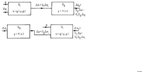
FIGURE 10.4. A general feedback loop. Either box may involve some parameters.

FIGURE 10.5. Regulation of the breathing rate. A change of metabolic rate (parameter p) causes a change in ventilation rate y, so that x = PCO2 does not change as much.

feedback loop, Fig. 10.4. To find the operating point, these two equations must be solved simultaneously. The easiest way to do this is to plot them on the same graph as in Fig. 10.5. When p = 60 mmol min−1, the operating point is at A. In a plot like this the horizontal axis represents the independent variable for one process and the dependent variable for the other.

If the feedback loop includes several variables, for example

x = f (w), y = g(x), z = h(y), w = i(z),

we can combine three of these equations to get x = F (y) and plot it with y = g(x).

We now have two processes relating the steady-state values of x and y. For alveolar gas exchange, we know x as a function of y: x = g(y, p). For the regulatory mechanism, we know y = f (x). Together, these constitute a

We can also see from Fig. 10.5 how feedback causes y to change in response to a change in parameter p to reduce the change in x. If y does not change, a change of p from 60 to 80 causes the operating point to go from A to B.

258 10. Feedback and Control

FIGURE 10.6. The open loop gain is calculated by opening the loop at any point. (a) Loop opened in y. (b) Loop opened in x.

In fact, y increases so that the new operating point is at D. The feedback loop is said to regulate the value of x.

The gain of a box is the ratio of the change in the output variable to the change in the input variable. For the first box in Fig. 10.4,

The product G1G2 is called the open-loop gain (OLG). Its name comes from the fact that if the feedback loop is opened at any point and a small change is made in the input variable at the opening, the change in the output variable is the open-loop gain times the change in the

The open-loop gain can be calculated by taking the derivatives in either order, which corresponds to breaking the loop after either box (Fig. 10.6).

If the relationships between the derivatives have been plotted as in Fig. 10.5, it may be easiest to evaluate the derivatives graphically. In that case, it is easiest to work with ∂y/∂x for box g. But ∂y/∂x = 1/(∂x/∂y). There-

It is important to calculate the gain in the direction that causality operates. Going around the loop the wrong way gives the reciprocal of the open-loop gain.

We can now calculate how much feedback reduces the change in x, compared to the case in which there is no feedback and the value of y going into box g is held fixed. For box g, where x = g(y, p), we can write for small

When there is feedback, there is a value of ∆y to be included. If the change in x with feedback is ∆x , the change in y can be calculated from the second box:

∂f

∆y = (10.10)

∂x

This can be combined with Eq. 10.9:

The e ect of feedback is to cause a change in y which reduces the change in x by the factor 1 − OLG. When the feedback is negative, the open-loop gain is negative, 1 − OLG is greater than one, and there is a reduction in ∆x. If the feedback is positive and the open-loop gain is less than one, ∆x is larger than ∆x.

For the respiration example, the equations for each box

If p changes from 60 to 62, then without feedback ∆x = (0.757)(2) = 1.5. With feedback, ∆x = 1.5/(1 + 5.48) = 0.23.

10.4Approach to Equilibrium without Feedback

The technique described in the preceding section allows us to determine the equilibrium state or operating point of a system if we can measure the functions f and g. It does not tell us how the system behaves when it is not at the equilibrium point, nor does it tell us how the system moves from one point to another when parameter p is changed. To learn that, we need an equation of motion for each process or box in the feedback loop. The equation of motion is usually a di erential equation. In real systems the di erential equation is often nonlinear and di cult to solve. We first consider models described by linear di erential equations, and then we consider some of the behaviors of nonlinear systems.

The response of a system cannot be infinitely fast. At equilibrium the rate of exhaling carbon dioxide is the same as the rate of production throughout the body. If the rate of production rises in a certain muscle group, the extra carbon dioxide enters the blood and is distributed throughout the body, and the carbon dioxide concentrations in the blood and alveoli rise gradually.

To develop a quantitative model, assume that all the carbon dioxide in the body is stored in a single wellstirred compartment of volume Vc. This assumption of uniform concentration is certainly an oversimplification. The total number of moles is n and the concentration is n/Vc. The concentration in the blood is related to the partial pressure in the alveoli by a solubility constant α: n/Vc = αx. Therefore dn/dt = αVcdx/dt. Moreover, dn/dt is equal to the rate of production (Eq. 10.2) minus the rate of removal (Eq. 10.3):

We change the definition of F to take account of the fact that o and p are both the rate of oxygen consumption in slightly di erent units (o is in mol s−1 and p is in mmol min−1):

This di erential equation depends on both x and y and in fact is nonlinear since the variables are multiplied together in the last term. At equilibrium dx/dt = 0 and Eq. 10.14 gives Eq. 10.4.

If y is constant (a constant breathing rate, which could be accomplished by placing the subject on a respirator), then there is no feedback and Eq. 10.14 is a linear di erential equation with constant coe cients:

dx + y0 − b x = F p . dt αVcRT αVc

It can be solved using the techniques of Appendix F. Suppose that for t ≤ 0, p = p0, x = x0, and y = y0. For t > 0

the subject exercises, so that p = p0 + ∆p, x = x0 + ξ, and y is unchanged. The equation then becomes

The homogeneous equation is

where the time constant is

The homogeneous solution is ξ = Ae−t/τ1 . The particular

solution is

ξ = F RT ∆p = a ∆p, y0 − b

so the complete solution is ξ = a ∆p + Ae−t/τ1 . We now use the initial condition to determine A. At t = 0 ξ = 0, so A = −a ∆p. The complete solution without feedback that matches the initial condition is

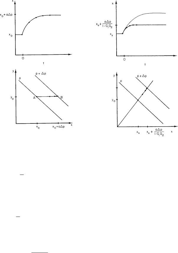
Figure 10.7 shows how x changes with time on a plot of x vs. t and a plot of y vs x. The dots are spaced at equal times.

10.5Approach to Equilibrium in a Feedback Loop with One Time Constant

Suppose now that y is allowed to change and that η = y − y0. We can write the equation for the change in x, Eq. 10.14 as

Multiplying all terms by τ1 as defined in Eq. 10.17, and identifying

260 10. Feedback and Control

FIGURE 10.7. The change in x without feedback in response to a step change in parameter p. (a) Plot of x vs t. (b) Plot of y vs x.

The product ξη in the last term makes the equation nonlinear. If we assume that the last term can be neglected, we have a linear di erential equation

Now assume that the response of the second box is

If this is substituted in the linearized equation, Eq. 10.20, the result is

The steady-state solution before t = 0 is x0 = a p0/(1 − G1G2). At t = 0 the oxygen demand is changed to p0 + ∆p. The new steady-state (inhomogeneous) solution is ξ = a ∆p/(1 − G1G2) and the homogeneous solution is ξ = Ae−t/τ where the time constant is

(You can show this by dividing each term in Eq. 10.22 by τ1 and comparing it to the equation for exponential

FIGURE 10.8. The change in x with feedback in response to a step change in parameter p. (a) Plot of x vs t. The change in x without feedback is shown for comparison. (b) Plot of y vs x.

decay.) After combining the homogeneous and inhomogeneous solutions and using the initial condition ξ(0) = 0 to determine A, we obtain the final result:

This solution has the same form as Eq. 10.18. Both the total change in x and the time constant have been reduced by the factor 1/(1 − G1G2). The change in y can be determined from η = G2ξ. The new solution is plotted along with the old solution in Fig. 10.8. This plot is for a system in which the open-loop gain is G1G2 = −1.3. The time constant and the change in x are both reduced by 1/2.3.

It is important to realize that although the feedback reduced the time constant, it has not made x change faster. The curve of x(t) with feedback has always changed less than the curve without feedback, and it has always changed more slowly. The reduction in time constant occurs because x does not change as much with feedback present, so it reaches its asymptotic value more quickly.

FIGURE 10.9. Changes in x and y after a step change in parameter p. (a) The second time constant is negligible compared to the first; x and y move exponentially to their new equilibrium values. (b) The first time constant is negligible; the slow change in y means that there is no feedback at first. (c) The second stage anticipates the change in y that will be required; there is too much feedback at first.

This result assumes that box f has a negligible time constant. Applied to the respiratory example, it means that the carbon dioxide–sensing system responds rapidly compared to the time it takes for carbon dioxide levels within the blood to change after a change in p. Figure 10.9(a) repeats Fig. 10.8 and shows the changes in x and y resulting from a step change in p. When the second time constant is negligible, y is always proportional to x and the system moves back and forth along line AB.

The CO2 sensors actually take a while to respond. To see what e ect this might have, imagine the extreme case where the sensors are very slow compared to the change of carbon dioxide concentration in the blood. In that case, when p changes, y does not change right away. The system behaves at first as if there were no feedback, moving from point A to point C in Fig. 10.9(b). As the feedback slowly takes e ect, the system moves from C to B. When the exercise ends, the system moves to point D because the

FIGURE 10.10. Change of arterial PCO2 and alveolar ventilation in response to exercise. Note that x = PCO2 is in the upper graph and the ventilation rate y is in the lower graph, the opposite of Fig. 10.9. Reprinted from A. C. Guyton. Textbook of Medical Physiology, 9th ed. p. 569, c 1995, Saunders–Else- vier, Inc. with permission of Elsevier. Data are extrapolated to humans from dogs. The dog experiments are described in C. R. Bainton (1972). J. Appl. Physiol. 33: 778–787.

subject is breathing too hard. Then it finally moves from D back to A. The actual system behaves in a manner somewhere between these two extremes, as we will see in the next section.

Consider a third possibility, that a regulatory mechanism anticipates the increased metabolic demand. This might happen if we took deep breaths before we began to exercise, or if additional muscle movement signaled the respiratory control center before the carbon dioxide concentration had a chance to change. Suppose that such anticipation is the only feedback mechanism. With the initiation of exercise, y changes to its final value. The level of carbon dioxide has not yet built up, so the increased ventilation reduces x below its normal value. We can approximate this by point D in Fig. 10.9(c). As the increased activity drives x up, the system moves at constant y to point B. When the exercise stops, y drops immediately to the resting value, though carbon dioxide is still coming out of the muscles. The result is that x rises to point C before finally falling back to point A.

Figure 10.10 shows what actually happens in the control of respiration. There is a fast neurological control and a slower chemical control. The result is a combination of the processes in Figs. 10.9(a)–(c).

If we had not made the linear approximation we would not have been able to solve the equation, but the behavior would have been very similar. The nonlinear equation is obtained by substituting the equation for the second box, Eq. 10.21, in Eq. 10.19 instead of Eq. 10.20. The resulting

FIGURE 10.11. Plots of τ1(dξ/dt) vs ξ. The straight dashed line is the linear approximation, Eq. 10.22. The parabolas are plots of the nonlinear equation, Eq. 10.25, for two di erent values of parameter a∆p. The closed circles show stable fixed points.

Both this and the linear version are plotted in Fig. 10.11 for a ∆p = 0. In each case dξ/dt is positive when ξ < 0 and negative when ξ > 0, so ξ approaches zero as time goes on. The direction of evolution of ξ is shown by the arrows on the nonlinear curve. This is often called a one-dimensional flow. The variable ξ “flows” to the origin, which is called a stable fixed point of the flow. If we change a ∆p to 10, the curve shifts as indicated by the dotted line, and the fixed point moves to a slightly di erent value of ξ.

This is a particular case of a di erential equation in one dependent variable of the form

dxdt = f (x).

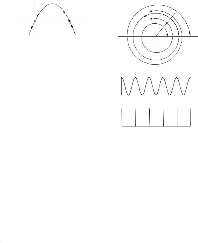
A great deal about the solution to the general equation can be learned by graphing it as we have done above. When the derivative is positive the function increases with time, and when it is negative it decreases. Figure 10.12(a) shows a more complicated function, with arrows showing the direction of the flow. The stable fixed point is indicated by a solid circle. There are two unstable fixed points, indicated by open circles. If x has precisely the value of an unstable fixed point, it remains there because dx/dt = 0. However, if it is displaced even a small amount, it flows away from the unstable point. Figure 10.12(b) shows just the x axis with the fixed points and the arrows. Stable fixed points are often called attractors

FIGURE 10.12. A more complicated flow on the line is shown.

(a) Plot of dx/dt vs x. The arrows show the direction that x changes. The open circles show unstable fixed points, and the filled circle is a stable fixed point. (b) The fixed points and the direction of flow are shown on the x axis.

or sinks. The unstable fixed points are called repellers or sources. Chapter 2 of Strogatz (1994) has an excellent and detailed discussion of one-dimensional flows.

10.6A Feedback Loop with Two Time Constants

In the preceding section we considered a feedback loop in which only one process had a significant time constant. The other process responded “instantaneously;” its time constant was much shorter. Here we consider the case in which both processes have comparable time constants. We will see that it is possible for such a (linear) system to exhibit damped sinusoidal behavior in response to an abrupt change in one of the parameters. Whether it does or not depends on the relative values of the two time constants and the open-loop gain. We consider both graphical and analytical techniques for solving this problem.

In earlier sections we discussed control of breathing. Equation 10.20 was the linear model for the departure of one variable from equilibrium:

dξ

τ1 dt = −ξ + G1η + a ∆p.

For the second process, instead of η = G2ξ we assume that the behavior is given by an analogous equation

For negative feedback either G1 or G2 must be negative. We have a special case of a pair of first-order di erential

equations

(Here x1 and x2 are general variables and have no relationship to the breathing problem considered earlier.)

We first combine the two first-order equations to make a second-order equation which, because we are using linear equations, can be solved exactly. To do this, di erentiate Eq. 10.20:

To eliminate η, solve Eq. 10.20 for G1η and substitute it in this equation:

(10.28) This is another linear di erential equation with constant coe cients. The right-hand side is a known function of time, since p(t) is known. The homogeneous equation is very common in physics and is called the harmonic oscillator equation. It is usually written in the form

Appendix F shows that as long as α ≥ ω0, the system is critically damped or overdamped and there will be no oscillation or “ringing.” This will be the case if

This equation is symmetric in τ1 and τ2. The important parameter is x = τ1/τ2. There is no ringing when

(1 + x)2 ≥ 1 − G1G2. 4x

Since the feedback is negative, G1G2 = − |G1G2|. Then there is no ringing if

If the two time constants are equal (x = 1), the righthand side of Eq. 10.31 is zero. There will be ringing if the open-loop gain has a magnitude greater than zero. For large values of x (say x > 10), the equation is approximately |G1G2| < x/4. If the magnitude of the open-loop gain is larger than this, there will be ringing.

We can see the general behavior of Eqs. 10.20 and 10.26 by examining the behavior of the derivatives. Both derivatives are zero and there is a fixed point when

For ∆p = 0 the fixed point is at the origin. Figures 10.13 and 10.14 show plots of ξ and η for di erent values of the gain and damping. The plots of η vs ξ are called statespace plots or phase-space or phase-plane plots. The plots shown here spiral to the fixed point. Depending on the values of the gains and time constants (try positive feedback) there can also be exponentially growing solutions. An extensive literature exists analyzing stability for both Eqs. 10.27 and their linearized versions. See Chapters 5 and 6 of Strogatz (1994) or Chapter 3 of Hilborn (2000).

10.7Models Using Nonlinear Di erential Equations

We have used many models in this book. In Chapter 2 we introduced a linear di erential equation that leads to exponential growth or decay. We used it to model tumor and bacterial growth and the movement of drugs through the body. We briefly examined some nonlinear extensions of this model. In Chapter 4, we modeled di usion processes with linear equations—Fick’s first and second laws—and we used a linear model to describe solvent drag. In Chapter 5, we used the model of a right-cylindrical pore. In Chapter 6, we used both a linear model—electrotonus— and a nonlinear model—the Hodgkin–Huxley equations. In this chapter we introduced a linear model for feedback, and we saw how two linear processes in a feedback loop could lead to oscillations, the linear harmonic oscillator.

Linear models have one advantage: they can be solved exactly. But most processes in nature are not linear. Jules-Henri Poincar´e realized around 1900 that systems described exactly by the completely deterministic equations of Newton’s laws could exhibit wild behavior.

Poincar´e was studying the three-body problem in astronomy (such as sun–earth–moon). While we are all familiar with the fact that the motion of the sun–earth–moon system is evolving smoothly with time and that eclipses can be predicted centuries in advance, this smooth behavior does not happen for all systems. For certain ranges of parameters (such as the masses of the objects) and initial positions and velocities, the solutions can exhibit behavior that is now termed chaotic. If we consider the motion that results from two sets of initial conditions that di er from each other only by an infinitesimal amount in one of the variables, we find that in chaotic behavior there can be solutions that diverge exponentially from each other as time goes on, even though the solutions remain bounded. Poincar´e developed some geometrical techniques for studying the behavior of such systems. Thorough study of nonlinear systems requires the use of a digital computer. As a result, it has only been since the 1970s that we have realized how often chaotic behavior can occur in a system governed by deterministic equations. With computers we have gained more insight into the properties of chaotic behavior.

Just as the harmonic oscillator provides a model for behavior seen in many contexts from electric circuits to shock absorbers in automobiles to the endocrine system, certain features of nonlinear models have wide applicability. These include period doubling, the ability to reset the phase (timing) of a nonlinear oscillator, and deterministic chaos.

Some have said that Newtonian physics has been overthrown by chaos. This is not true. The same equations hold; predictable motions with which we have long been familiar still take place. Much of our current technology is based on them. We build television sets and send a spacecraft to explore several planets in succession. With chaos, we have come to understand a rich set of solutions

to these same equations that we were not equipped to study before.

Many books about nonlinear systems have been written. A particularly interesting one for this audience is by Kaplan and Glass (1995). It is written for biologists and has many clear and relevant examples. Others are by Glass and Mackey (1988), by Hilborn (2000), and by Strogatz (1994).

Space limitations prevent more than a brief hint at some of the features of nonlinear dynamics, here and in Chapter 11. In this section we will discuss some oneand two-dimensional nonlinear di erential equations. These will not lead to chaos, but will allow us to describe a very simple model for phase resetting. In Sec. 10.8 we will discuss equations that exhibit chaotic behavior.

10.7.1Describing a Nonlinear System

Suppose that a nonlinear system with N variables can be described by a set of first-order di erential equations:

(These are an extension of the pair of di erential equations we saw as Eqs. 10.27. Our model of breathing had two variables. It would be more realistic to use a breathing model with more variables, since alveolar ventilation also depends on arterial pH, weakly on oxygen partial pressure, and on the nervous factors that were described earlier.)

η

If the equations are cast in this form with N variables, then N initial conditions are required, corresponding to the constant of integration required for each equation. It is customary to say that there are N degrees of freedom. This is the language of system dynamics. This definition of degrees of freedom is di erent from what we used in Chap. 3, where each degree of freedom was represented by a second-order di erential equation (d2x/dt2 = Fx/m, for example) and two initial conditions were required for each degree of freedom.

We can put Newton’s second law in this form by writing two first-order di erential equations instead of one second-order equation. For motion in one dimension, instead of

d2x

m dt2 = F (x, v), we write a pair of first-order equations:

This system has two degrees of freedom in our new terminology. In either description, two initial conditions are required.

In many situations the force (or more generally the function on the right-hand side of Eqs. 10.32) is time dependent. In standard form, the functions on the right do not depend on time. This is remedied by introducing one more variable, xN +1 = t. The additional di erential equation is dxN +1/dt = 1.

The evolution or “motion” of the system can be thought of as a trajectory in N -dimensional space, starting from the point that represents the initial conditions.

Time is a parameter. We have seen an example of this for two dimensions in Figs. 10.13 and 10.14. It is possible to prove that two distinct trajectories cannot intersect in a finite period of time and that a single trajectory cannot cross itself at a later time [see Hilborn (2000, p. 77) or Strogatz (1994, p. 149).] This is true in the full N - dimensional space; if we were to measure only two variables, we could see apparent intersections in the state plane that we were observing. This means that chaotic behavior, in which variables appear to change wildly and two-dimensional trajectories appear to cross, does not occur for a pair of di erential equations of the form in Eqs. 10.32. At least three variables are required. A system with two degrees of freedom that is externally driven2 can exhibit chaotic behavior because of the additional variable xN +1 that is introduced.

10.7.2An Example of Phase Resetting: The Radial Isochron Clock

In Chapter 2 we studied the logistic di erential equation

It is convenient to rewrite the logistic equation in terms of the dimensionless variable x = y/y∞:

2That is, one of the functions on the right-hand side of the set of equations depends on time.

266 10. Feedback and Control

dx/dt

FIGURE 10.15. Plot of dx/dt vs x for the logistic di erential equation.

This separates the scale factor y∞ from the dynamic factor b that tells how rapidly y and x are changing.3 A plot of dx/dt vs x is shown in Fig. 10.15. There is an unstable fixed point at x = 0 and a stable fixed point at x = 1. The logistic equation is one of a whole class of nonlinear first-order di erential equations for which dx/dt as a function of x has a maximum. It has been studied extensively because of its relative simplicity, and it has been used for population modeling. (Better models are available.4 The logistic model assumes that the population is independent of the populations of other species, that the growth of the species does not a ect the carrying capacity y∞, and that the population increases smoothly with time.)

Many of the important features of nonlinear systems do not occur with one degree of freedom. We can make a very simple model system that displays the properties of systems with two degrees of freedom by combining the logistic equation for variable r with an angle variable θ that increases at a constant rate:

This has the form of Eqs. 10.32. We can interpret (r, θ) as the polar coordinates of a point in the xy plane. When t has increased from 0 to 1 the angle has increased from 0 to 2π, which is equivalent to starting again with θ = 0. This system has been used by many authors. Glass and Mackey (1988) have proposed that it be called the radial isochron clock. Typical behavior is shown in Fig. 10.16(a). If r = 1 there is a circular orbit corresponding to the stable fixed point of Eq. 10.33. Such a stable orbit is called a stable limit cycle.5 There is an unstable limit cycle, r = 0, corresponding to the unstable fixed point of Eq. 10.33. Any initial conditions except r = 0 give trajectories that move toward the stable circular limit cycle as time progresses. The set of points in the xy plane lying on orbits that move to the limit cycle as t → ∞

3We could also, if we wish, define a new time scale, t = bt, and deal with the completely dimensionless equation dx/dt = x(1 −x).

4See Begon et al. (1996).

5A stable limit cycle is an oscillation in the solutions to a set of di erential equations that is always reestablished following any small perturbation.

r

θ

(c)

FIGURE 10.16. A system with two degrees of freedom. (a) The limit cycle is represented by the solid circle. Systems starting elsewhere in the plane have trajectories that approach the limit cycle as t → ∞, as shown by the dashed lines. (b) The value of x = r cos θ is plotted as a function of time. (c) A timing pulse is generated every time θ is a multiple of 2π.

is called the basin of attraction for the limit cycle. In this case the basin of attraction includes all points except the origin. If we look at the time behavior, Fig. 10.16(b) shows the behavior of x = r cos θ on the limit cycle. The oscillator might provide timing information as the phase moves through some value. Figure 10.16(c) shows a series of pulses every time θ is a multiple of 2π.

In many cases the di erential equations contain one or more parameters that can be varied, and the number and shape of the limit cycles change as the parameters are changed. A point in parameter space at which the number of limit cycles changes or their stability changes is called a bifurcation. We will see examples of bifurcations in the next section. See the references for a much more extensive discussion.

One important characteristic of nonlinear oscillators is that a single pulse can reset their phase. If they are subject to a series of periodic pulses they can be entrained to