

Intermediate Physics for Medicine and Biology - Russell K. Hobbie & Bradley J. Roth
.pdfSymbol |
Use |
Units |
First |
|
|
|
used on |
|
|
|
page |
0 |
Permittivity of free |
N−1 m−2 |
178 |
|
space |
C2 |
|
λ |
Space constant |
m |
193 |
σ, σi, σo |
Electrical conduc- |
S m−1 |
178 |
|
tivity |
|
|
ρ |
Charge density |
C m−3 |
190 |
τ |
Time constant |
s |
193 |
θ |
Angle |
|
180 |
ξ |
Ratio of x to R |
|
184 |
Ω |
Solid angle |
|
181 |
Problems 197
Section 7.2
Problem 4 Modify the closing argument of Sec. 7.2 by considering electrodes that are disks rather than spheres. (Hint: The capacitance you will need is given in Sec. 6.19.)
Problem 5 Suppose an axon is surrounded by a thin layer of extracellular fluid of thickness d. Use arguments based on the intracellular resistance to estimate the ratio ∆vo/∆vi in this case.
Problems
Section 7.1
Problem 1 A single nerve or muscle cell is stretched along the x axis and embedded in an infinite homogeneous medium of conductivity σo. Current i0 leaves the cell at x = b and enters the cell again at x = −b. Find the current density j at distance r from the axis in the x = 0 plane.
Problem 2 An axon is stretched along the x axis. At one instant of time an impulse traveling along the axon has the form shown in the graph. The electrical conductivity inside the axon of radius a is σi. In the infinite external medium it is σo. Find an expression for the potential at point (x0, y0).
|
|
|
|
|
v |
|
|
|
|||
|
|
|
|
|
|
0 |
|||||
|
|
|
|
|
|
|
|
|
|
|
|
|
|
|
|
|
|
|
|
|
|
|
|
|
|
|
|
|
x |
||||||
|
|
|
|
|
|
|
|
|
|
|
|
-2b |
0 |
b |
|||||||||
Problem 3 The interior potential of a cylindrical cell is plotted at one instant of time. Distances along the cell are given in terms of length b. The cell has radius a and electrical conductivity σi. The resting potential is 0 and the depolarized potential is v0. The conductivity of the external medium is σo.
(a) Find expressions for, and plot, the current along the cell in the four regions (x < 0, 0 < x < 2b, 2b < x <
3b, 3b < x).
(b) Find the potential at a point (x, y) outside the cell in terms of the parameters given in the problem. The point is not necessarily far from the cell.
Section 7.3
Problem 6 Starting with Eq. 7.4, make the Taylor’s series expansions described in the text, and use them to derive Eq. 7.16.
Problem 7 What would be the current-dipole moment of a nerve cell of radius 2 µm when it depolarizes? Would myelination make any di erence? Does the result depend on the rise time of the depolarization? If the impulse lasts 1 ms and the conduction speed is 5 m s−1, how far apart are the rising and falling edges of the pulse?
Problem 8 An axon or muscle cell is stretched along the x axis on either side of the origin. As it depolarizes, a constant current dipole p pointing to the right sweeps along the axis with velocity u. An electrode at (x = 0, y = a) measures the potential with respect to v = 0 at infinity. Ignore repolarization. Find an expression for v at the electrode as a function of time and sketch it. Assume that at t = 0, p is directly under the electrode at x = 0.
 Observation Point
a
p
x 
Problem 9 An electrode at (x = 0, y = a) measures the potential outside an axon with respect to v = 0 at infinity. A nerve impulse is at point x along the axon, measured from the perpendicular from the electrode to the axon. At x + b a current dipole points to the right, representing the depolarization wave front. At x − b a vector of the same magnitude points to the left,representing repolarization. Obtain an expression for v as a function of x, b, p, and a. Plot it in the case a = 1, b = 0.05.
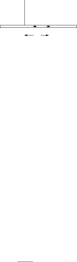
198 7. The Exterior Potential and the Electrocardiogram
 ELECTRODE
a
-p p
 x-b
x-b  x+b
x+b
Section 7.5
Problem 15 Suppose a wave front propagates at a speed of 0.25 m s−1and its refractory period lasts 250 ms. Calculate the minimum path length of its reentrant circuit. Most reentrant wave fronts are somewhat slower and briefer than this, so their paths may be shorter.
Section 7.7
Problem 10 A dipole p located at the origin (0, 0, 0) is oriented in the x direction. The potential vo(x) produced by this dipole is measured along the line y = 0, z = d.
(a)Find an equation for vo(x) in terms of x, d, σo (the conductivity of the medium) and the dipole strength, p.
(b)Find an expression for the depth d of the dipole in terms of the distance ∆x, defined as the distance between the minimum and maximum of vo(x, y). This is an example of an “inverse problem,”in which you try to learn about the source (in this case, the depth of p) from measurements of vo.
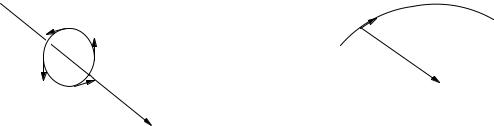
Problem 11 The “solid angle theorem” is often used to interpret electrocardiograms. The relationship between the exterior potential and the solid angle in Eq. 7.15 is a general result: the potential is proportional to the solid angle subtended by the wave front. Use this result to explain
(a) why a closed wave front produces no exterior potential, and (b) why an open wave front produces a potential that depends only on the geometry of its opening or rim.
Section 7.4
Problem 12 Run the program of Fig. 7.11 and plot the potential for di erent distances from the axon.
Problem 13 Modify the program of Fig. 7.11 to calculate the potential from a single Gaussian action potential and plot the potential.
Problem 14 Let the intracellular potential be zero except in the range −a < x < a, where it is given by
|
2 |
a + x |
2 |
|||||
|
, |
|||||||
|
|
|
|
|
|
|
|
|
|
|
|
|
a |
|
|
|
|
|
|
|
|
|
|
|
|
|
|
|
|
|
|
x |
|
2 |
|
|
|
|
|
|
|
|
|
|
|
|
|
|
|
|
|
||
vi = |
1 − 2 |
|
|
|
, |
|||
a |
|
|
||||||
|
|
a |
|
x |
2 |
|||
|
|
− |
|
|||||
|
2 |
|
|
|
|
|
, |
|
|
|
|
|
|
|
|||
|
|
|
|
|
|
|
|
|
|
|
|
|
|
|
|
|
|
|
|
|
|
a |
|
|
|
|
−a < x < −a/2
−a/2 < x < a/2
a/2 < x < a.
Plot vi vs x. Use Eq. 7.21 to calculate the exterior potential at (x0, y0). You may need the integral
|
√ |
dx |
= sinh− |
1 x |
||
|
|
|
b |
. |
||
|
x2 + b2 |
|||||
Problem 16 Two electrodes are placed in a uniform conducting medium 10 cm from a cell of radius 5 µm and 10 cm from each other, so that the two electrodes and the cell form an equilateral triangle. When the cell depolarizes the potential rises 90 mV. What will be the potential di erence between the two electrodes when the cell orientation is optimum? How many cells would be needed to give a potential di erence of 1 mV between the electrodes? Assume σi/σo = 10.
Problem 17 Guess whatever parameters you need to predict the voltage at the peak of the QRS wave in lead II. Compare your results to the electrocardiogram of Fig. 7.23.
Problem 18 At a particular instant of the cardiac cycle, p is located at the midpoint of a line connecting two electrodes that are 50 cm apart, and p is parallel to that line. At that instant the magnitude of the potential di erence between the electrodes is 1.5 mV. Upon depolarization, the potential change within the cells has magnitude 90 mV.
(a)What is the magnitude of p?
(b)If σi/σo = 10, what is the cross-sectional area of the advancing region of depolarization?
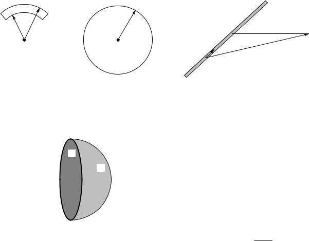
Problem 19 A semi-infinite slab of myocardium occupies the region z > 0. A hemispherical wave of depolarization moves radially away from the origin through the slab. At some instant of time the radius of the hemispherical
depolarizing wavefront is R. Assume that p = dp, that dp is everywhere perpendicular to the advancing wavefront, and that the magnitude of dp is proportional to the local area of the wavefront. Find p. Assume that the observation point is very far away compared to R.
Problem 20 Make measurements on yourself and construct Fig. 7.19.
Problem 21 Experiments have been done in which a dog heart was stimulated by an electrode deep within the myocardium. No exterior potential di erence was detected until the spherical wave of depolarization grew large enough so that part of it intercepted one wall of the heart. Why?
Problem 22 Prove directly from Eq. 7.31 that I − II + III = 0. (It is sometimes said that the equilateral nature of Einthoven’s triangle is necessary to prove this.)
Problem 23 Derive Eqs. 7.32.
Section 7.8
Problem 24 Estimate the lower limit for the duration of the QRS complex by calculating the time required for a wave front to propagate across the heart wall. Assume the wall thickness is 10 mm and the propagation speed is 0.2 m s−1.
Problem 25 In an ECG recording, the width of one large square corresponds to 200 ms. A normal heart rate is between 60 and 100 beats min−1. The heart rate is usually measured by counting the number of large squares between adjacent QRS complexes.
(a)How many large squares are there for a normal heart rate?
(b)In Fig. 7.30 determine the rate of the atria and of the ventricles.
Problem 26 Consider Lead II of the normal ECG in Fig. 7.23. The QRS wave and the T wave are both positive. Use a one-dimensional model to convince yourself that the QRS complex and the T wave should have opposite polarities. Why then is the T wave inverted? Find a way to explain the inverted T wave by letting the action potential duration vary between epicardium (outside) and endocardium (inside). On which surface should the duration be longest?
Section 7.9
Problem 27 Ohm’s law says that j = σE. Draw what j and E look like (a) in a circuit consisting of a battery and a resistor; (b) for the current flowing when a nerve cell depolarizes.
Problem 28 Obtain the values for β for a cube of length a on a side, for a cylinder of radius a and length h, and for a sphere of radius a.
Problem 29 Show that Eq. 7.36a is the same as Eq. 6.51 by considering the interior of a single cell stretched along the x axis as in Fig. 6.28. Consider the charge in a small cylindrical region of axoplasm of length h and radius a, the cylindrical surface of which is surrounded by cell membrane. Show that the total charge Q within the axoplasm changes according to
∂Q |
= πa2h |
∂ρi |
= C |
∂vm |
|
+ im |
||||||||||
|
∂t |
|
|
|
|
∂t |
||||||||||
|
|
|
∂t |
|
|
|
|
|
|
|
|
|||||
|
|
|
= 2πah cm |
∂vm |
|
+ jm , |
||||||||||
|
|
|
|
|
|
|||||||||||
|
|
|
|
|
|
|
|
∂t |
|
|
|
|||||
and that this can be combined with Eq. 7.36a to give |
||||||||||||||||
|
cm |
∂vm |
+ jm = |
|
πa2h |
σi |
∂2vi |
|
||||||||
|
|
|
|
|
∂x2 |
|||||||||||
|
|
|
∂t |
|
2πah |
|||||||||||
|
|
|
= |
|
σia |
|
∂2vi |
, |
||||||||
|
|
|
|
|
|
|||||||||||
|
|
|
|
|
|
|
|
2 ∂x2 |
|
|
|
|||||
which is the same as Eq. 6.51, except that it is written in terms of σi, a, and h instead of a and ri.
Problems 199
Problem 30 Clark and Plonsey (1968) solved Eq. 7.37 for a cylindrical axon of radius a using the following method. Assume that the potentials all vary in the z direction sinusoidally, for instance vm(z) = V sin(kz), where
Vis a constant.
(a)Show that the intracellular and extracellular potentials can be written as
vi = AI0(kr) sin(kx) |
|
vo = BK0(kr) sin(kz), |
(7.53) |
where In and Kn are “modified Bessel functions” obeying the equation
1 |
|
∂ |
|
|
∂v |
|
|
2 |
+ |
n2 |
|
|
|
|
|
r |
|
− |
k |
|
|
v = 0. |
|
r ∂r |
|
∂r |
|
r2 |
|||||||
(b) Determine the constants A and B in terms of V , using the following two boundary conditions: vm = vi −vo, and σi(∂vi/∂r) = σo(∂vo/∂r), both evaluated at r = a. You will need to use the Bessel function identities dI0(kr)/dr = kI1(kr) and dK0/dr = −kK1(kr). Clark and Plonsey used this result and Fourier analysis (Chapter 11) to determine vi and vo when they are not sinusoidal in z.
Problem 31 Starting with the bidomain equations, divide Eq. 7.44a by σix and 7.44b by σex. Now subtract one equation from the other. Under what conditions do the equations contain vm = vi −vo but not vi and vo individually?
Section 7.10
Problem 32 Verify Eq. 7.47.
Problem 33 Verify the values given for rheobase and chronaxie in Table 7.1 that are based on Table 6.1.
Problem 34 An approximation to the error function is given by Abramowitz and Stegun (1972)
erf(x) ≈ 1 − 1 + 0.278393x + 0.230389x2 + 0.000972x3 + 0.078108x4 −4, x > 0.
Calculate erf(x) using this approximation for x = 0, 0.5, 1.0, 2.0 and ∞. Using trial and error, determine the value of x for which erf(x) = 0.5. (See Eq. 7.50.)
Problem 35 Find the equivalent of Eq. 7.45 in terms of the charge required for the stimulation.
Problem 36 If the medium has a constant resistance, find the energy required for stimulation as a function of pulse duration.
Problem 37 A typical pacemaker electrode has a surface area of 10 mm2. What is its resistance into an infinite medium if it is modeled as a sphere? If it is modeled as a disk? (You will have to use results from Chapter 6 and assign a value for σo.)

200 7. The Exterior Potential and the Electrocardiogram
Problem 38 Equation 6.51 is the cable equation for a nerve axon. Assume that the axon membrane is passive [jm = gm(vi − vo), where gm is a constant].
(a) Express the equation in terms of vm and vo instead of vi and vo, where vm = vi − vo.
(b) Divide the resulting equation by gm, and then write
the cable equation in terms of the time constant cm/gm
√
and the length constant 1/ 2πarigm.
(c) Put all the terms containing vm on the left side, and terms containing vo on the right side. The resulting equation should look like Eq. 6.55, except for a new source term on the right side equal to −λ2∂2vo/∂x2. (Measure vm with respect to resting potential so vr = 0 in Eq. 6.55). The negative of this new term has been called the “activating function” (Rattay, 1987). It is useful when studying electrical stimulation of nerves.
Problem 39 For this problem, use the activating function derived in Problem 38. Assume that λ and τ are negligibly small, so that vm simply equals the activating function. Consider a point electrode in an infinite, homogeneous volume conductor at distance d from the axon. The extracellular potential vo is vo = (1/4πσo) I/r.
(a)Calculate vm as a function of position x along the axon (x = 0 is the closest position to the electrode).
(b)Assume that the axon will fire an action potential
if vm somewhere along the axon is greater than Vthreshold. Calculate the ratio of the stimulation current I needed to excite the axon for a cathode (negative electrode) and an anode (positive electrode).
Problem 40 For this problem, use the activating function derived in Problem 38. An action potential can be excited if a stimulus depolarizes an axon to a value greater than Vthreshold, and a propagating action potential can be blocked if a stimulus hyperpolarizes to a value of vm less
than −Vblock(Vblock > Vthreshold).
(a)For a cathodal electrode [vo = (1/4πσo) I/r] calculate the ratio of the threshold current to the ratio of the current needed to block propagation.
(b)Use two electrodes (one cathodal and one anodal) to design a stimulator that will result in one-way propagation along the axon (say, propagation only in the positive x direction, but blocked in the negative x direction). For an application of such electrodes during functional electrical stimulation, see Ungar et al. (1986).
Problem 41 For this problem, use the activating function derived in Problem 38, and block by hyperpolarization derived in Problem 40. The factor of λ2 in the activating function implies that larger diameter axons are easier to stimulate than smaller diameter axons. Sometimes you want to excite the smaller fibers without the larger fibers (“physiological recruitment”). Describe qualitatively how you can use a single electrode and block in the hyperpolarized region to obtain physiological recruitment. For a more complete discussion, see Tai and Jiang (1994).
Problem 42 In “second degree” heart block, the wave front sometimes passes through the conduction system and sometimes does not. Qualitatively sketch the ECG for a heart with second degree block for at least five beats. Specifically include the case where every third wave is blocked. Include the P wave, the QRS wave, and the T wave.
Problem 43 During “sinus exit block” the SA node functions normally but the wave front fails to propagate from the SA node to the atria. Sketch five beats of an ECG with all beats normal except the third, which undergoes sinus exit block.
Problem 44 In “sick sinus syndrome” the SA node has a slow and erratic rate. The AV node and conduction system function properly. You plan to implant a pacemaker in the patient. Should it stimulate the atria or the ventricles? Why?
Problem 45 A patient with “intermittent heart block” has an AV node which functions normally most of the time with occasional episodes of block, lasting perhaps several hours. Design a pacemaker to treat the patient. Ideally, your design will not stimulate the heart when it is functioning normally. Describe
(a)whether you will stimulate the atria or ventricles
(b)which chambers you will monitor with a recording electrode
(c)what logic your pacemaker will use to determine when to stimulate. Your design may be similar to a “demand pacemaker” described in Je rey (2001), p. 132.
Problem 46 The |
Lapicque |
strength-duration (SD) |
|||||||||||||
curve is |
|
|
i |
|
|
|
tC |
|
|
|
|
||||
|
|
|
|
|
|
= 1 + |
, |
|
|
|
|||||
|
|
|
|
|
iR |
|
|||||||||
|
|
|
|
|
|
|
t |
||||||||
the SD curve in terms of the error function is |
|||||||||||||||
|
i |
|
|
|
|
|
1 |
|
|
|
|
|
|||
|
|
|
= |
|
|
|
|
|
, |
||||||
iR |
erf # |
|
|
|
|||||||||||
|
0.228t/tC |
||||||||||||||
and the SD curve derived in Ch. 6 Prob. 35 is |
|||||||||||||||
|
|
|
i |
= |
|
|
1 |
|
. |
|
|||||
|
iR |
|
|
|
|
|
|
||||||||
|
1 |
− e−0.693t/tC |
|||||||||||||
(a)Plot all three curves for 0 < t/tC < 5. Use the equation in Problem 34 to evaluate the error function.
(b)Find approximations for each curve for t/tC 1.
You may need the Taylor’s series expansions ex ≈ 1 + x
√
and erf(x) ≈ 2x/ π.
(c) Discuss the physical assumptions that were used to derive each curve.
Problem 47 Consider a pacemaker delivering 2 mA, 1 V, 1 ms pulse every second. Pacemakers are often powered by a lithium-iodide battery that can deliver a total charge of 2 ampere hours.

(a)What is the energy per pulse?
(b)What is the average power?
(c)How long will the battery last?
(d)Your answer to (c) is an overestimate of battery lifetime, in part because the battery voltage begins to decline before all its charge has been delivered, and in part
because the pacemaker circuitry requires a small, constant current. For this pacemaker, add a constant current drain of 5 µA and assume that the useful lifetime of the battery is over when 75% of the total charge has been delivered. How long will the battery last in this case?
Section 7.11
Problem 48 When measuring the EEG with electrodes distributed according to the 10–20 system, you obtain measurements of the potential di erence between the ith electrode (i = 1, . . . , 20) and the reference electrode (i = 21). Show that by computing the average reference vi =
20
(vi − v20) − (1/20) j=1 (vj − v20) , the resulting values of vi are independent of the reference potential v21.
Problem 49 Consider a very simple model of the EEG: a dipole p pointing in the z direction at the center of a spherical conductor of radius R and conductivity σo. The potential vo can be written as the sum of two terms: the potential of a dipole in an unbounded medium plus a potential that obeys Laplace’s equation
p cos θ
vo = 4πσor2 + Ar cos θ
where r and θ are in spherical coordinates, and A is an unknown constant.
(a)Use Appendix L to show that the second term in the expression for vo obeys Laplace’s equation.
(b)If the region outside the spherical conductor is air (an insulator), determine the value of A by using the boundary condition that the radial current at the surface of the sphere is zero.
(c)Calculate vo as measured at the sphere surface (r = R), and determine by what factor vo di ers from what it would be in the case of an unbounded volume conductor.
Problem 50 Suppose you measure the EEG potential vj at N locations rj = (xj , yj , zj ), j = 1, . . . , N . Assume vj is produced by a dipole p = (px, py , pz ) located at the origin. Define
N |
|
2 |
|
|
|
pxxj + py yj + pz zj |
|
R = j=1 |
|
− vj , |
|
4πσ xj2 + yj2 + zj2 3/2 |
|||
which measures the least-squares di erence between the data and the potential predicted by a single-dipole model. (Chapter 11 explores the least-squares method in greater detail.) The goal is to find the dipole components px, py , pz that fit the data best (minimize R).
References 201
(a)Minimize R with respect to px (set dR/dpx = 0) and find an equation relating px, py , and pz .
(b)Repeat for py and pz .
(c)Write the three equations in the form Ap = b, where A is a 3 × 3 matrix and b is a 3 × 1 vector. Find expressions for the components of A and b.
(d)If we had not assumed that we knew the location of the dipole, the problem would be much more di cult. Assume the dipole is at location rp = (xp, yp, zp). Modify R and then try to minimize it with respect to rp. Carry the calculation far enough to convince yourself that you must now solve nonlinear equations to determine rp. Press et al. (1992) discuss methods for making nonlinear least squares fits.
References
Abramowitz, M., and I. A. Stegun. (1972). Handbook of Mathematical Functions with Formulas, Graphs, and Mathematical Tables. Washington, U.S. Government Printing O ce.
Antzelevitch, C., S. Sicouri, A. Lukas, V. V. Nesterenko, D-W. Liu, and J. M. Di Diego (1995). Regional di erences of electrophysiology in ventricular cells: physiological and clinical implications. In D. P. Zipes and J. Jalife, eds. Cardiac Electrophysiology: From Cell to Bedside, 2nd ed. Philadelphia, Saunders, pp. 228–245.
Barold, S. S. (1985). Modern Cardiac Pacing. Mount Kisco, NY, Futura.
Campbell, D. L., R. L. Rasmusson, M. B. Comer, and H. C. Strauss (1995). The cardiac calcium-independent transient outward potassium current: kinetics, molecular properties, and role in ventricular repolarization. In D. P. Zipes and J. Jalife, eds. Cardiac Electrophysiology: From Cell to Bedside, 2nd ed. Philadelphia, Saunders, pp. 83– 96.
Clark, J. and R. Plonsey (1968). The extracellular potential field of a single active nerve fiber in a volume conductor. Biophys. J. 8: 842–864.
Davidenko, J. M. (1995). Spiral waves in the heart: Experimental demonstration of a theory. In D. P. Zipes and J. Jalife, eds. Cardiac Electrophysiology: From Cell to Bedside, 2nd ed. Philadelphia, Saunders, pp. 478– 488.
Delmar, M., H. S. Du y, P. L. Sorgen, S. M. Ta et and D. C. Spray (2004). Molecular organization and regulation of the cardiac gap junction channel connexin43. In D. P. Zipes and J. Jalife, eds. Cardiac Electrophysiology: From Cell to Bedside, 4th ed. Philadelphia, Saunders, pp. 66–76.
Geddes, L. A., and J. D. Bourland (1985). The strength-duration curve. IEEE Trans. Biomed. Eng. 32: 458–459.
Gulrajani, R. M. (1998) Bioelectricity and Biomagnetism. New York, Wiley.
202 7. The Exterior Potential and the Electrocardiogram
Harris, J. W., and H. Stocker (1998). Handbook of Mathematics and Computational Science. New York, Springer.
Henriquez, C. S. (1993). Simulating the electrical behavior of cardiac tissue using the bidomain model. Crit. Rev. Biomed. Eng. 21(1): 1–77.
Je rey, K. (2001). Machines in Our Hearts. Baltimore, Johns Hopkins University Press.
Knisley, S. B., B. C. Hill, and R. E. Ideker (1994). Virtual electrode e ects in myocardial fibers. Biophys. J. 66: 719–728.
Lapicque, L. (1909). Definition experimentale de l’excitabilite. Comptes Rendus Acad. Sci. 67(2): 280–283.
Lindemans, F. W. and J. J. Denier van der Gon (1978). Current thresholds and liminal size in excitation of heart muscle. Cardiovasc. Res. 12: 477–485.
Malmivuo, J., and R. Plonsey (1995). Bioelectromagnetism. Oxford, Oxford University Press.
Miller, C. E. and C. S. Henriquez. (1990). Finite element analysis of bioelectric phenomena. Crit. Rev. Biomed. Eng. 18(3): 207–233.
Mitrani, R. D., L. S. Klein, D. P. Rardon, D. P. Zipes and W. M. Miles (1995). Current trends in the implantable cardioverter–defibrillator. In D. P. Zipes and J. Jalife, eds. Cardiac Electrophysiology: From Cell to Bedside, 2nd ed. Philadelphia, Saunders, pp. 1393–1403.
Moses, H. W., B. D. Miller, K. P. Moulton, and J. A. Schneider (2000). A Practical Guide to Cardiac Pacing.
5th ed. Philadelphia, Lippincott Williams and Wilkins. Neunlist, M. and L. Tung (1995). Spatial distribution
of cardiac transmembrane potentials around an extracellular electrode: Dependence on fiber orientation. Biophys. J. 68: 2310–2322.
Nunez, P. L. and R. Srinivasan (2005). Electric Fields of the Brain. 2nd. ed. Oxford, Oxford University Press.
Oudit, G. Y., R. J. Ramirez and P. H. Backx (2004). Voltage-regulated potassium channels. In D. P. Zipes and J. Jalife, eds. Cardiac Electrophysiology: From Cell to Bedside, 4th ed. Philadelphia, Saunders, pp. 19–32.
Plonsey, R. (1969). Bioelectric Phenomena. New York, McGraw-Hill.
Press, W. H., S. A. Teukolsky, W. T. Vetterling, and B. P. Flannery (1992). Numerical Recipes in C: The Art of Scientific Computing, 2nd ed., reprinted with corrections, 1995. New York, Cambridge University Press.
Rardon, D. P., W. M. Miles, and D. P. Zipes (2000). Atrioventricular block and dissociation. In D. P. Zipes and J. Jalife, eds. Cardiac Electrophysiology: From Cell to Bedside, 3rd ed. Philadelphia, Saunders, pp. 451–459.
Rattay, F. (1987) Ways to approximate currentdistance relations for electrically stimulated fibers. J. Theor. Biol. 125: 339–349.
Rosenbaum, D. S. and J. Jalife (2001). Optical Mapping of Cardiac Excitation and Arrhythmias. Armonk, NY, Futura.
Roth, B. J. (1992). How the anisotropy of the intracellular and extracellular conductivities influences stimulation of cardiac muscle. J. Math. Biol. 30: 633–646.
Roth, B. J. (1994). Mechanisms for electrical stimulation of excitable tissue. Crit. Rev. Biomed. Eng. 22(3/4): 253–305.
Roth, B. J. (1997). Electrical conductivity values used with the bidomain model of cardiac tissue. IEEE Trans. Biomed. Eng. 44: 326–328.
Roth, B. J. and J. P. Wikswo, Jr. (1994). Electrical stimulation of cardiac tissue: A bidomain model with active membrane properties. IEEE Trans. Biomed. Eng. 41(3): 232–240.
Rudy, Y. and J. E. Burnes (1999). Noninvasive electrocardiographic imaging. Ann. Noninvasive Electrocardiol.
4(3): 340–359.
Sepulveda, N. G., B. J. Roth, and J. P. Wikswo, Jr. (1989). Current injection into a two-dimensional anisotropic bidomain. Biophys. J. 55: 987–999.
Stanley, P. C., T. C. Pilkington, and M. N. Morrow (1986). The e ects of thoracic inhomogeneities on the relationship between epicardial and torso potentials. IEEE Trans. Biomed. Eng. 33(3): 273–284.
Tai, C., and D. Jiang (1994). Selective stimulation of smaller fibers in a compound nerve trunk with single cathode by rectangular current pulses. IEEE Trans. Biomed. Eng. 41: 286–291.
Trayanova, N., C. S. Henriquez, and R. Plonsey (1990). Limitations of approximate solutions for computing extracellular potential of single fibers and bundle equivalents. IEEE Trans. Biomed. Eng. 37(1): 22– 35.
Ungar, I. J., J. T. Mortimer, and J. D. Sweeney (1986). Generation of unidrectionally propagating action potentials using a monopolar electrode cu . Ann. Biomed. Eng. 14: 437–450.
Voorhees, C. R., W. D. Voorhees III, L. A. Geddes, J. D. Bourland, and M. Hinds (1992). The chronaxie for myocardium and motor nerve in the dog with surface chest electrodes. IEEE Trans. Biomed. Eng. 39(6): 624– 628.
Watanabe, A., and H. Grundfest (1961). Impulse propagation at the septal and commisural junctions of crayfish lateral giant axons. J. Gen. Physiol. 45: 267–308.
Wikswo, J. P., Jr. (1995). Tissue anisotropy, the cardiac bidomain, and the virtual cathode e ect. In D. P. Zipes and J. Jalife, eds. Cardiac Electrophysiology: From Cell to Bedside, 2nd ed. Philadelphia, Saunders, pp. 348– 361.
8
Biomagnetism
The field of biomagnetism has exploded in recent decades. Magnetic signals have been detected from the heart, brain, skeletal muscles, and isolated nerve and muscle preparations. Measurements of the magnetic susceptibility of the lung show the e ect of dust inhalation. Susceptibility measurements of the heart can determine blood volume, while the susceptibility of the liver can measure iron stores in the body. Bacteria and some animals contain aggregates of magnetic particles, often attached to neural tissue. Bacteria use these magnetic particles to determine which way is down. Magnetism is used for orientation by birds and other animals.
Sections 8.1 and 8.2 review the basics of magnetism. Section 8.3 calculates the magnetic field of an axon in an infinite conducting medium. This result, which shows that the field is due primarily to the current dipole in the interior of the axon, is approximately true for the magnetocardiogram and evoked responses from the brain, described in Secs. 8.4 and 8.5.
Section 8.6 reviews electromagnetic induction. Section 8.7 describes the use of varying magnetic fields to stimulate nerves or muscles. Section 8.8 introduces diamagnetic, paramagnetic, and ferromagnetic materials and describes biomagnetic e ects that depend on magnetic materials. Section 8.9 reviews instrumentation for measuring these weak magnetic signals.
8.1The Magnetic Force on a Moving Charge
Lodestone, compass needles, and other forms of magnetism have been known for centuries, but it was not until 1820 that Hans Christen Oersted showed that an electric current could deflect a compass needle. We now know that magnetism results from electric forces that moving
charges exert on other moving charges and that the appearance of the magnetic force is a consequence of special relativity. An excellent development of magnetism from this perspective is found in Purcell (1985). The development here is more traditional and is incomplete.
Suppose that a beam of electrons is accelerated in a cathode-ray tube (as in an oscilloscope, computer display, or television receiver) and causes a spot of light to be emitted where it strikes a fluorescent screen. The electron source is cathode C in Fig. 8.1. The accelerating electrode is E. The fact that the beam is accelerated toward a positively charged electrode confirms that the electrons are negatively charged. The beam normally strikes the screen at point X. Placing a battery between plates A and B creates an electric field that deflects the beam as it passes between the plates. If plate A is positively charged, the beam is deflected upward to point Y . If the battery is removed and the north pole of a bar magnet is brought to the position shown, the beam is deflected to point Z.
We say that a magnetic field exists in the space surrounding the bar magnet and that the direction of the magnetic field at any point is the direction a small compass needle located there would point. Experiment shows that the force is at right angles to both the direction of the magnetic field and the velocity of the charged particle. Detailed experiments show that the magnitude of the force F is proportional to the charge, the magnitude of the velocity v, and the strength of magnetic field B. (In fact, modern definitions of the magnetic field are based on this proportionality.) The magnitude of the force is greatest when v and B are perpendicular. We have seen a relationship like this between three vectors before: the vector product or cross product, which was associated with torque and defined in Sec. 1.4. We write
F = q(v × B). |
(8.1) |

204 8. Biomagnetism
C
E
A
B Y
X
(a)
C
S
N
E
Z X
(b)
FIGURE 8.1. An electron beam generated at cathode C and accelerated through electrode E strikes the fluorescent screen on the right. (a) A positive charge on plate A and negative charge on plate B deflects the beam from X to Y . (b) A bar magnet brought close as shown deflects the beam to point Z.
The SI unit of B is the tesla, T. An earlier name was the weber per square meter. The cgs unit is the gauss, G: 1 T = 104 G. If a coordinate system is set up so that v is along the x axis and B is along the y axis, then v ×B and the force on a positive charge are along the +z axis. For negatively charged electrons F is in the opposite direction. Combining Eq. 8.1 with the electric force gives the full expression for the electromagnetic force, often called the Lorentz force:
F = q(E + v × B). |
(8.2) |
FHE FHE
|
|
|
|
|
|
|
|
|
|
|
|
|
|
|
|
|
|
|
|
|
|
|
|
|
|
|
E |
|
|
|
a |
|
|
H |
|
|
|
|
|
|
|
|
|
|
|
|
m |
|
|||||
|
|
|
|
m |
|
|
|
|
|
|
|
|
||||||||||||||
|
|
|
|
|
|
|
|
|
|
|
|
|
|
|||||||||||||
|
|
|
|
|
|
|
|
|
|
|
|
|
|
|
|
|
|
|
|
|
|
|
|
|
||
|
|
|
|
|
|
|
|
|
|
|
|
|
|
|
|
|
|
|
|
|
|
|
|
|
||
|
|
|
|
|
|
|
|
|
|
|
b |
|
|
|
|
|
|
|
θ |
|
|
|
||||
|
|
|
|
|
|
|
|
|
|
|
|
|
|
|
|
|
|
|
|
|
|
|
|
|
|
|
EF |
|
|
|
|
|
|
|
|
θ |
|
|
|
|
|
|
F |
|
|
|
|
|
|
|
|||
F |
|
|
b |
|
|
|
|
|
|
|
|
|
|
GH |
|
b |
|
|
|
|
|
|||||
|
|
|
φ |
|
|
|
φ |
|
B |
|||||||||||||||||
|
|
|
|
|
|
|
|
|
|
|
|
|
|
|
||||||||||||
|
|
|
|
|
|
|
|
|
|
|
|
|
|
|
||||||||||||
|
|
|
|
|
|
|
|
|
|
|
|
|
|
|
|
|||||||||||
|
|
|
|
|
|
|
|
|
|
|
|
|
|
|
|
|
|
|
|
|||||||
|
|
F |
|
|
a |
G |
|
|
|
B |
|
|
|
|
|
|
||||||||||
|
|
|
|
|
|
|
i |
|
|
|
|
|
|
|
|
|
|
|
||||||||
|
|
|
|
|
|
|
|
|
|
|
|
|
|
|
|
|
|
|
|
|
|
|
|
|
|
|
|
|
|
|
|
|
|
|
FFG |
|
|
|
|
|
|
FFG |
|
|
|
||||||||
|
|
Perspective view |
|
|
|
|
|
Side view |
|
|
|
|||||||||||||||
FIGURE 8.2. A current-carrying loop is in a uniform magnetic field. The dashed line from the center of the loop to the center of edge F G, vector B and vector m all lie in the same plane. The sum of angles θ and φ is π/2. The forces on opposite sides add to zero. There is a torque on the loop unless its plane is perpendicular to the field (φ = π/2). The magnetic moment m is perpendicular to the plane of the loop.
Since current in a wire is the result of moving charges, there is a force on a segment of wire carrying a current. Suppose that there are C particles per unit volume, each with charge q, drifting with speed v along a segment of wire of length ds and cross-sectional area S. In time dt the total charge passing a given plane is CvqS dt [see Eq. 4.11] so that the current is i = CvqS. If there is a magnetic field perpendicular to the wire, the magnitude of the force on each particle is qvB and the total force is CS ds qvB = iB ds. If vector ds is defined along the wire in the direction of the positive current, then the contribution to the magnetic force from this segment of the wire is
dF = i(ds × B). |
(8.3) |
If a small rectangular loop of wire is placed in a uniform magnetic field and a current is made to flow in the wire, there is a magnetic force on each arm of the loop. (The current can be led to and from the rectangle by two parallel closely spaced wires, in which the forces cancel because the currents are in opposite directions. Forces not considered here maintain the position of the loop.)
Figure 8.2 shows the orientation of the loop in the horizontal magnetic field. The magnetic moment m is perpendicular to the loop and makes an angle θ with the direction of B. Sides HE and F G are of length a and perpendicular to the field. The other two sides have length b. The force on side EF has magnitude iBb sin φ and is directed as shown. Side GH has a force of equal magnitude in the opposite direction. On side F G the force is down and on side HE it is up, both with magnitude iBa. The vector sum of all the forces is zero. There is a torque, however. If the torque is taken about the center of the loop, the F G force and HE force each exert a torque of magnitude (iBa)(b/2) cos φ. The total torque is therefore iBab cos φ. The loop is said to have a magnetic moment m of magnitude iS, where S = ab is the area of the loop. Vector m is defined to point perpendicular to the loop in
8.2 The Magnetic Field of a Moving Charge or a Current |
205 |
d s
θ
B
B
i
FIGURE 8.3. The magnetic field around a current-carrying wire is at right angles to the wire and the perpendicular from the observation point to the wire. The magnitude is inversely proportional to the distance from the wire.
the direction of the thumb of the right hand when the fingers curl in the direction of the current around the loop. The units of m are A m2 or J T−1. In terms of angle θ between m and B, the torque τ exerted by the magnetic field on the magnetic moment has magnitude iabB sin θ, so
τ = m × B. |
(8.4) |
The torque is zero when m and B are parallel or antiparallel. When they are parallel the equilibrium is stable: if there is a small rotation of m the torque acts to return it to equilibrium. When they are antiparallel, the equilibrium is unstable.
A small current loop can be used to test for the presence of a magnetic field. At equilibrium m points in the same direction that a small compass needle would point and gives the direction of B. Measuring the torque for a known displacement of m from this direction gives the magnitude of B.
8.2The Magnetic Field of a Moving Charge or a Current
8.2.1The Divergence of the Magnetic Field Is Zero
FIGURE 8.4. The line integral of B · ds is calculated by multiplying ds by the component of B parallel to ds, that is B cos θ.
Close to the wire B is always at right angles to the wire, in contrast to the electric field, which close to a charge always points toward or away from it. In the electric case, the flux of E through a closed surface is proportional to the charge within the volume enclosed by the surface (Gauss’s law). In contrast, the flux of B through a closed surface is always zero. In the notation of Sec. 4.1,
|
|
B · dS = 0. |
|
|
Bn dS = |
(8.6) |
|
closed surface |
closed surface |
|
|
If single magnetic charges (magnetic monopoles) existed, the flux would be proportional to the magnetic charge within the volume. Magnetic monopoles have never been observed, in spite of considerable e ort to find them.
As in the electric case, we can construct lines of B. The tangent to the line always points in the direction of B. For the long wire, the lines of B are circles. One can show from Eq. 8.6 that lines of B always close on themselves.
Equation 8.6 has the form of the continuity equation, Eq. 4.4, with B substituted for j and with C = 0. The di erential version of Eq. 8.6 can therefore be obtained from Eq. 4.8. It is
div B = · B = 0. |
(8.7) |
With a compass needle or small sensing coil we can in principle map the magnetic field surrounding a bar magnet or a wire carrying a current. If we examine the field near a long straight wire carrying current i, we find that B is always at right angles to the wire and at distance r has magnitude
B = |
µ0i |
. |
(8.5) |
|
|||
|
2πr |
|
|
The constant µ0 is analogous to 0 in electrostatics and is exactly 4π × 10−7 T m A−1 (or Ω s m−1). Figure 8.3 shows the direction of B at various locations around a wire. The direction of the force is consistent with Eq. 8.2 if the direction of B is defined to be the direction in which the fingers of the right hand curl when the thumb points along the wire in the direction of the (positive) current.
8.2.2 Ampere’s Circuital Law
It is also interesting to consider the line integral of B around a closed path. That is, for any element of the path ds shown in Fig. 8.4 take the projection of B in the direction of ds, B cos θ. Sum up all the contributions B cos θ ds along the entire closed path. For path ABCD in Fig. 8.5(a), the result is zero. The reason is that B cos θ ds is zero on segments AB and CD. On segment DA it is (µ0i/2πa)(aφ) = µ0iφ/2π, while on segment BC it is −(µ0i/2πb)(bφ) = −µ0iφ/2π. In Fig. 8.5(b) the path is circular with the wire at the center, and the line integral is B(2πa) = µ0i. This result is general:
/ |
/ |
(8.8) |
B cos θ ds = |
B · ds = µ0i. |
206 8. Biomagnetism
A |
|
|
D |
B |
|
a |
C |
b |
φ |
a |
|
|
|
|
|
|
Wire |
|
Wire |
(a) (b)
FIGURE 8.5. Two paths of integration. In (a) the path does
not encircle the wire carrying the current, and |
0 |
B · ds = 0. |
||||
In (b) the path encircles the wire and |
0 |
B |
· |
ds = µ0i. |
||
|
||||||
S |
|
x = 0 |
a |
P |
|
|
|
|
dx |
θ |
r |
|
FIGURE 8.7. The Biot–Savart law is used to calculate the magnetic field at point P due to an infinite wire.
4.4, shows that the flux of j (the total current) through any closed surface is zero. Two surfaces S and S , both bounded by the path, form a closed surface as shown in Fig. 8.6. The total current through surface S is the same as the total current through S .
S' |
8.2.3 The Biot-Savart Law |
|
Bounding
Path
FIGURE 8.6. Since the total current or flux of j through any closed surface is zero, the current through surface S is equal to the current through surface S .
The circle on the integral sign means that the integral is taken around a closed path. The line integral of the magnetic field around a closed path is equal to µ0 times the current through a circuit enclosed by that path. If two wires carrying equal and opposite currents are enclosed by the path of the line integral, the integral is zero. It does not mean that B is zero everywhere on the path.
A more general statement is that for steady currents the line integral of B around a closed path is equal to the integral of the current density j through any surface enclosed by the path:
/ |
|
(8.9) |
B · ds = µ0 |
j · dS. |
This is known as Ampere’s circuital law. Like Gauss’s law, it is always true but not always useful. It is true for currents that do not vary with time, but it can be used to calculate the magnetic field only if symmetry can be used to argue that B is always parallel to the path and has the same magnitude at all points on the path.
The surface used to calculate the right-hand side can be any surface bounded by the path used on the left. Since we are dealing with steady currents for which there is no charge accumulation, the continuity equation, Eq.
In situations where the symmetry of the problem does not allow the field to be calculated from Ampere’s law, it is possible to find the field due to a steady current in a closed circuit using the Biot–Savart law. The contribution dB to the magnetic field from current i flowing along a line element ds is
dB = |
µ0i |
|
ds × r |
. |
(8.10) |
|
|
||||
|
4π r3 |
|
|||
Vector r is from the current element to the point where the field is to be calculated. The field is found by integrating over the entire circuit.
Figure 8.7 shows how this integration is done for an infinitely long straight wire along the x axis. The contribution at point P is obtained by dropping a perpendicular from P to the wire to define x = 0. The distance from P to the wire is a. The contribution from an element dx at point x is
dB = |
µ0i dx sin θ |
= |
µ0i |
|
a dx |
. |
||
|
|
|
|
|
||||
4π r2 |
|
|
||||||
|
|
4π r3 |
||||||
Since r2 = a2 + x2 the total field is
B = |
µ0i |
∞ |
a dx |
|
|
|
|
|
|||
|
4π −∞ (a2 + x2)3/2 |
∞ |
|
|
|
|
|||||
= |
µ0ia |
|
|
x |
|
= |
|
µ0i |
. |
||
4π a2(x2 + a2)1/2 |
|
|
|||||||||
|
−∞ |
|
2πa |
||||||||
|
|
|
|
|
|
|
|
|
|
|
|
This agrees with Eq. 8.5 and the result obtained using Ampere’s circuital law.
A steady current from a point source that spreads uniformly in all directions generates no magnetic field. To see why, consider Fig. 8.8. The source of current is at O. The magnetic field at P can be calculated using the Biot– Savart law. For any element ds a symmetric element ds