Intermediate Physics for Medicine and Biology - Russell K. Hobbie & Bradley J. Roth

FIGURE 6.3. Ion concentrations in a typical mammalian nerve and in the extracellular fluid surrounding the nerve. Concentrations are in mmol l−1; co/ci is the concentration ratio. The membrane thickness is b.

chemical [Nolte (2002), p. 193, Guyton and Hall (2000, Chapter 45)]. In electrical synapses, channels connect the interior of one cell with the next. In the chemical case a neurotransmitter chemical is secreted by the first cell. It crosses the synaptic cleft (about 50 nm) and enters the next cell.

At the neuromuscular junction the transmitter is acetylcholine (ACh). ACh increases the permeability of nearby muscle to sodium, which then enters and depolarizes the muscle membrane. The process is quantized.2 Packets of acetylcholine of definite size are liberated [Katz (1966, Chapter 9); Patton et al. (1989, Chapter 6)].

There are a number of neurotransmitters in the central nervous system. Glutamate is a common excitatory neurotransmitter in the central nervous system. It increases the membrane permeability to sodium ions, which enhances depolarization. Glycine, on the other hand, is an inhibitory neurotransmitter. It causes the interior potential becomes more negative (hyperpolarized) and firing is inhibited. A number of other chemical mediators such as norepinephrine, epinephrine, dopamine, serotonin, histamine, aspartate, and gamma-aminobutyric acid, are also found in the nervous system [Guyton and Hall (2000, Chapter 45)].

If the potential becomes high enough (that is, more positive or less negative), the regenerative action of the membrane takes over, and the cell initiates an impulse. If the input end of the cell acts as a transducer, the interior potential rises when the cell is stimulated. If the input is from another nerve, the signal may cause the potential to increase by a subthreshold amount so that two or more stimuli must be received simultaneously to cause firing, or it may decrease the potential and inhibit stimulation by another nerve at the synapse. This makes possible the logic network that comprises the central nervous system.

2See Problem 3 in Appendix J.

FIGURE 6.4. Force F is exerted by charge q1 on charge q2. It points along a line between them. An equal and opposite force −F is exerted by q2 on q1.

6.2Coulomb’s Law, Superposition, and the Electric Field

Coulomb’s law relates the electrical force between two objects to their electrical charge and separation. For our purpose, Coulomb’s law is a summary of many experiments. If two objects have electrical charge q1 and q2, respectively, and are separated by a distance r, then there is a force between them, the magnitude of which is given by

When the charge is measured in coulombs (C), F in newtons (N), and r in meters (m), the constant has the value

to an accuracy of 0.1%.3 The direction of the force is along the line between the two charges as shown in Fig. 6.4. If the charges are both positive or both negative, the force is repulsive, which is consistent with assigning a positive sign to F. If one is positive and the other negative, then the force is attractive, and F has a negative value. Force F is exerted by charge q1 on charge q2. The force exerted by q2 on q1 has the same magnitude but points in the opposite direction. The forces on both charges act to separate them if they have the same sign and to attract them if the signs are opposite.

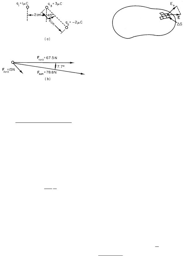
If two or more charges exert a force on the particular charge being considered, the total force is found by applying Coulomb’s law to each charge (paired with the one on which we want to find the force) and adding the vector forces that are so calculated. An example of this is shown in Fig. 6.5. Charges q1, q2, and q3 are +1.0 ×10−6, −2.0 × 10−6, and +3.0 × 10−6 C, respectively. The magnitude of the force that q1 exerts on q3 is

3The quantity 1/4π 0 has been assigned the exact value 8.987551787368176 4 × 109. This is because in 1983 the velocity

of light, c, was defined to be exactly 299, 792, 458 m s−1 and 1/4π 0 ≡ 10−7c2.

138 6. Impulses in Nerve and Muscle Cells

FIGURE 6.5. An example of applying Coulomb’s law and adding forces on q3 due to charges q1 and q2. (a) The arrangement of charges. (b) The forces on q3.

Similarly, the force exerted by q2 on q3 is

The minus sign means that the force is attractive, that is, toward q2. The two forces are shown in Fig. 6.5b, along with their vector sum. The sum can be found by components as in Chap. 1. The result is 78.8 N at an angle of 7.7 ◦ clockwise from the direction of F1 on 3.

If a collection of charges causes a force to act on some other charge (a “test charge”) located somewhere in space, we say that the collection of charges produces an electric field at that point in space. One can think, for example, of charge q1 producing an electric field vector, of magnitude

pointing radially away from q1 (if q1 is positive) or radially toward q1 (if q1 is negative). The force on test charge q2 placed at the observing point is then

6.3 Gauss’s Law

It is possible to derive a theorem about the electric field from a collection of charges, known as Gauss’s law. Rather than derive it from Coulomb’s law, we will state it and show that Coulomb’s law can be derived from it. Then we will consider some examples of its use.

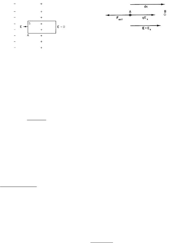
Divide up any closed surface into elements of surface area, such as ∆S in Fig. 6.6. For each element ∆S, calculate the component of E normal to the surface, En,

FIGURE 6.6. Calculating the integral of the normal component of E through a surface.

and multiply it by the magnitude of the surface area ∆S. Add these quantities for the entire closed surface, calling them positive if the normal component of E points outward and negative if E points inward. Gauss’s law says that the resulting sum is equal to the total charge inside the surface, divided by 0. In symbols,4

This surface integral is exactly the same as the flux of the continuity equation, Eq. 4.4. It is in fact called the electric field flux.5

While Gauss’s law is always true, it is not always useful. It is helpful only in cases where E is constant over the entire surface of integration, or when the surface can be divided into smaller surfaces, on each of which En can be argued to be constant or zero. One of the few cases in which Gauss’s law is useful to calculate E is the case of a point charge, and another is related to the cell membrane. In each case, the symmetry of the problem allows the surface of integration to be specified so that En is either constant or zero.

The first example is a point charge in empty space. Since such a charge has no preferred orientation (it is a point), and since there is nothing else around to specify a preferred direction in space, the electric field must point radially toward or away from the charge and must depend only on distance from the charge. Therefore, if the surface of integration is a sphere centered on the charge, En is the same everywhere on the sphere. It can be taken outside

The integral of dS over the entire surface of the sphere is just the surface area of the sphere, 4πr2 (see Appendix L). Gauss’s law gives

4πr2E = q0

4Some books use one integral sign in this equation and others use two. Strictly speaking the integral over a surface is a twodimensional integral.

5Additional discussion and examples can be found in Schey (1997).

FIGURE 6.7. Gauss’s law is used to calculate the electric field from an infinite line of charge. The Gaussian surface is a segment of a cylinder concentric with the line of charge.

or

q

E = 4π 0r2 .

Gauss’s law implies Coulomb’s law for the case of a point charge.

If the charge in this problem is not a point charge, nothing changes in the argument as long as the charge distribution is spherically symmetric. The electric field at a distance r from the center of the distribution is the same as if all the charge within the sphere of radius r were located at the center of the sphere.

Next, consider a problem with cylindrical symmetry rather than spherical symmetry. An example is an infinitely long line of charge. For a segment of the line of charge of length L, the amount of charge is proportional to L, q = λL, where λ is the linear charge density in units C m−1. Symmetry shows that E must point radially outward (or inward) and be perpendicular to the line. Therefore if the Gaussian surface is a cylinder of length L and radius r, the axis of which is the line of charge, one can argue that on the end caps En = 0, while on the wraparound surface of the cylinder En = |E|. This is shown in Fig. 6.7. The total integral is therefore the integral for the

wraparound surface, which is E dS. The surface area of the cylinder is its circumference (2πr) times its length (L). Therefore Gauss’s law becomes 2πrL E = λL/ 0, or

Since the constant 1/4π 0 is so easily remembered, it is convenient to write this as

Consider next an infinite sheet of charge, with charge per unit area σ C m−2. The symmetry of the situation requires that E be perpendicular to the sheet. To see why, suppose that E is not perpendicular to the sheet. I stand on the sheet looking in such a direction that E points diagonally o to my left. If I turn around in place, I see E pointing diagonally o to my right. Since the charge

FIGURE 6.8. A portion of an infinite sheet of charge and the appropriate Gaussian surface.

per unit area is constant and extends an infinite distance in every direction, the charge distribution looks exactly the same as it did before I turned around. The only way to resolve this contradiction (that E changed direction while the charge distribution did not change) is to have E perpendicular to the sheet.

The Gaussian surface can be a cylinder with end caps of area S and sides perpendicular to the sheet. Let the end caps be a distance a from the charge sheet on one side and b from the charge sheet on the other, as in Fig. 6.8. Since there is no component of E across the sides of the cylinder, changing b or a does not change the total flux through the surface. Since the charge inside the volume does not change, E must be independent of distance from the sheet of charge. (This is true only because the charge sheet is infinite.) By symmetry, the flux through each end cap is the same, as may be seen from the cross section of the surface in Fig. 6.9. The total flux is therefore 2ES, while the charge within the volume is σS. Therefore, Gauss’s law gives

There is, of course, something quite unreal about a sheet of charge extending to infinity. However, it is a good approximation for an observation point close to a finite sheet of charge. If the sheet is limited in extent and the observation point is far away, the distance to all parts of the sheet from the observation point is nearly the same, and the charge sheet may be regarded as a point charge. If one considers a rectangular sheet of charge lying in the xy plane of width 2c and length 2b, as shown in Fig. 6.10, it is possible to calculate exactly the E field along the z axis. By symmetry, the field points along the z axis. The surface charge density is σ. The distance is r =

x2 + y2 + z2 1/2. The component of E parallel to the z axis is E cos θ = Ez/r. Therefore, if the charge in element

140 6. Impulses in Nerve and Muscle Cells

FIGURE 6.9. A side view of the Gaussian surface in Fig. 6.8.

z

2b

2c

FIGURE 6.10. A rectangular sheet of charge. The electric field along the z axis is shown in Fig. 6.11 for 2b = 200 m and 2c = 2 m.

This integral can be evaluated (see Problem 7). The result is

This is plotted in Fig. 6.11 for c = 1 m, b = 100 m. Close to the sheet (z 1) the field is constant, as it is for an infinite sheet of charge. Far away compared to 1 m but close compared to 100 m, the field is proportional to 1/r as with a line charge. Far away compared to 100 m, the field is proportional to 1/r2, as from a point charge.

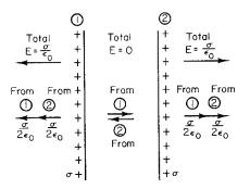
As a final example, consider two infinite sheets of charge, one with density −σ and the other with density +σ, as shown in Fig. 6.12. This can be solved by using the result for a single sheet of charge, Eq. 6.8, and the principle of superposition. Consider first the region I of Fig. 6.12. There, the negative charge will give an E field

FIGURE 6.11. A log-log plot of the electric field from a sheet of charge of width 2 m and length 200 m, measured along the perpendicular bisector of the sheet (Fig. 6.10). Much closer than 1 m, the field is constant. Around 10 m the field is proportional to 1/r, the field from a line charge. Farther away than 100 m the field is proportional to 1/r2, the field from a point charge.

that has magnitude σ/2 0 and points toward the right, while the positive sheet of charge will give an E field of σ/2 0 pointing to the left. The total E field in region I is zero. A similar argument can be made in region III with the field of the negative charge pointing left and that of the positive charge pointing to the right. Again the sum is zero. In region II, however, the two E fields point in the same direction, and the total field is

Notice the factor of 2 di erence between Eqs. 6.8 and 6.11. Another way to explain the di erence is that there is no E in region III, so that a Gaussian surface can be constructed as shown in Fig. 6.13. Then the flux is zero through every surface except cap A. The charge within

FIGURE 6.12. The electric field due to two infinite sheets of charge of opposite sign.

FIGURE 6.13. A Gaussian surface to determine the electric field between two sheets of charge.

the volume is σS, while the flux through cap A is ES. Therefore, E = σ/ 0.

Within a cell membrane of 6 nm thickness surrounding a cell of radius 5 µm or 5,000 nm, the electric field can be calculated by making the approximation that the sheets of charge are infinite. Suppose that the electric field within the membrane is 1.17 × 107 N C−1. (We will learn how to determine this value later.) From Eq. 6.11

This tells us something about the makeup of the cell. The membrane is in contact with atoms, each of which has a diameter of about 10−10 m. Therefore, there are approximately 1020 atoms (in water molecules, as ions, etc.) in contact with one square meter of the membrane surface.

Suppose that the excess charge that causes the electric field in the membrane resides in these atoms and that each atom is either neutral or a monovalent ion. The number of atoms in the square meter which are charged is

1014)/(1020) = 6.4 × 10−6. Roughly 1 in every 105 atoms in contact with the membrane carries an unneutralized charge. (This result is modified by partial neutralization of this external charge by charge movement within the membrane. See Eq. 6.35.)

6.4 Potential Di erence

It is often convenient to talk about the electrical potential di erence, or voltage di erence instead of the electric field. The potential is related to the di erence in energy of a charge when it is at di erent points in space. Suppose

FIGURE 6.14. A charge q is moved from A to B, a distance dx in the x direction. External force Fext keeps the charge from being accelerated.

that an electric field E of magnitude Ex points along the x axis. A positive charge is located at point A. A force Fext must be applied to the charge by something besides the electric field, or else the charge will be accelerated to the right by the force qEx. The charge can be moved slowly to the right at a constant speed so that its kinetic energy remains fixed, if the external force is always to the left and its magnitude is adjusted so that Fext = −qEx.

This situation is shown in Fig. 6.14. The external force does work on the charge. One can either say that the total work done on the charge by both forces is equal to zero, or one can ignore the work done by the electric force and invent the idea of potential energy—energy of position— due to the electric field. The increase in potential energy6 as the charge moves a distance dx is

dU = Fext dx = −qEx dx.

If Ex varies with position, the total change in potential energy when the particle is moved without acceleration from A to B is given by

For example, in a constant electric field of 1.4 × 107 N C−1, a particle with charge q = 1.6×10−19 C experiences an electric force equal to 2.24 × 10−12 N. If it is moved 5 nm along the x axis, the electric force does 1.12 × 10−20 J of work on it, increasing its kinetic energy. To prevent this increase in kinetic energy, Fext must be applied. The external force does work −1.12 × 10−20 J. We can either say that the total work done by both forces is zero or we can ignore the electrical force and say that the external force changed the potential energy of the particle by −1.12 × 10−20 J as the particle moved from A to B.

If the displacement of the particle is perpendicular to the direction of the electric field, it is also perpendicular to the direction of Fext. Therefore neither force does work on the particle and the potential energy is unchanged.

6In earlier chapters the potential energy was called Ep, and the total energy was called U . For the next few pages U will be used for potential energy, to avoid confusion with a component of the electric field.

142 6. Impulses in Nerve and Muscle Cells

This fact can be used to prove [Halliday et al. (1992, p. 652)] that in three dimensions,

Using the notation of a “dot” or scalar product of two vectors (Sec. 1.8), this can also be written as a line integral along any path from A to B:

It is easier to evaluate the integral along some paths than along others.

The potential energy di erence is measured in joules. It is always proportional to the charge of the particle that is moved in the electric field. It is convenient to define the potential di erence to be the potential energy di erence per unit charge. When the energy di erence is in joules and the charge is in coulombs, the ratio is J C−1, which is called a volt (V):

FIGURE 6.15. The electric field in and around an infinite plane conductor carrying a charge on each surface.

In many cases, it is customary to define the potential to be zero at infinity. Then the potential at point B is

B

v(B) = − Ex dx.

∞

If you try to apply this equation to the infinite line and sheet of charge, you will discover that it does not work. The reason is that you cannot get infinitely far away from a charge distribution that extends to infinity.

To move a charge of +3 C from point A to point B where the potential is 5 V higher requires that 15 J work be done on the charge. If the charge is then allowed to move back to point A under the influence of only the electric field, its kinetic energy increases by 15 J as the potential energy decreases by the same amount.

This definition of potential, when combined with the definition of potential energy, Eq. 6.12, gives

That is, the component of the electric field in any direction is the negative of the rate of change of potential in that direction. The units of E were seen earlier to be N C−1 (from F = qE). Equation 6.16 shows that the units of E are also V m−1. In three dimensions this relationship becomes

where grad is the gradient operation defined in Eq. 4.19. Notice that only di erences in potential energy and differences in potential (or colloquially, di erences in voltage) are meaningful. We can speak of the potential at a point only if we have previously agreed that the potential at some other point will be called zero. Then we are really speaking of the di erence of potential between the

reference point and the point in question.

6.5 Conductors

In some substances, such as metals or liquids containing ions, electric charges are free to move. When all motion of these charges has ceased and static equilibrium exists, there is no net charge within the conductor. To see why there is not, consider a small volume within the conductor. If there were an electric field within that region, the charges there would experience an electric force. Since they are free to move, this force would accelerate them. This force will vanish only when the electric field within the conductor is zero. Therefore, in the static case the electric field within a conductor is zero. Now apply Gauss’s law to a small volume within the conductor. Since the electric field in the conductor is zero everywhere, the flux through the Gaussian surface is zero, and the net charge within the volume is zero.

At the surface of the conductor, there may well be charge that gives rise to electric fields outside the conductor. Consider, for example, an infinite sheet of metal that has positive charge on it. The positive charge will distribute itself as shown in Fig. 6.15, and either superposition or Gauss’s law may be used to show that the electric field outside the conductor is σ/ 0.

Because the electric field is zero throughout a conductor in equilibrium, no work is required to move a charge from one point to another. All parts of the conductor are at the same potential. This statement is true only if the charges are not moving. We will see later that if they are (that is, if a current is flowing), then the electric field in

the conductor is not zero and the potential in the conductor is not the same everywhere.

6.6 Capacitance

Suppose that two conductors are fixed in space, with charge +Q on one and −Q on the other. The potential di erence v between the conductors is proportional to Q. The proportionality constant depends on the geometrical arrangement of the conductors. When the proportionality is written as

the proportionality constant C is called the capacitance. The units of capacitance are C V−1 or farads (F).

As an example of capacitance, consider two parallel conducting plates side by side. Let the area of each be S and the separation be b. The charge layers of Fig. 6.13 might be charge on the inner surface of each conductor. The total charge on each plate has magnitude σS. The electric field between the plates is σ/ 0 and the potential di erence is v = Eb = σb/ 0. (Note that the potential di erence is proportional to the charge per unit area.) The capacitance is

If the plates are separated further with a fixed charge on them, the potential di erence increases and the capacitance is decreased. Increasing the area and charge of the plates with fixed σ and fixed b increases Q and C but not v.

6.7 Dielectrics

Charges rearrange themselves so that there is no static electric field within a conductor. In a dielectric, charges are not free to move far enough to completely cancel the e ect of any external electric field, but they can move far enough to cause a partial cancellation.7

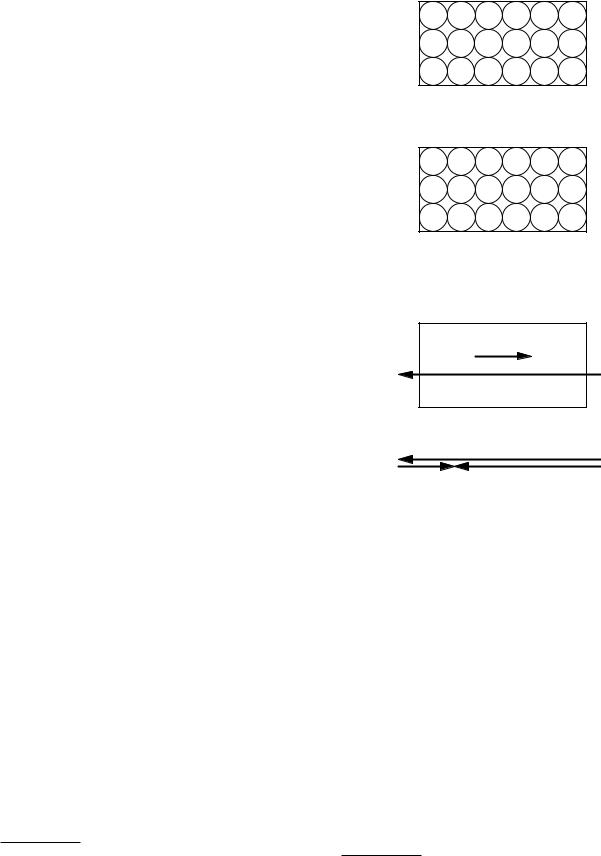
The partial neutralization of the external electric field can be understood from the following model. Consider a dielectric in the absence of external fields. The electron distribution of each atom is centered on the nucleus so that there is no electric field (at least when we average over a region containing many atoms). This is shown schematically in Fig. 6.16(a), in which each + sign represents a nucleus and each circle represents a distribution of negative charge in an atom.

7In some materials an electric field applied along one direction can cause charge displacement in a di erent direction. This book deals only with cases in which the induced electric field is parallel to the applied electric field.

(b)

Eext

(d)

FIGURE 6.16. The polarization of a dielectric by an external electric field. (a) Atoms in the absence of an external field. (b) An external electric field causes a shift of each electron cloud relative to the positively charged nucleus. (c) There is a net buildup of positive charge at the left edge of the dielectric and of negative charge at the right edge. (d) The total electric field within the dielectric is the sum of the external electric field and the polarization electric field induced in the dielectric.

Figure 6.16(b) shows some external charges producing an electric field. If the dielectric is introduced in the space where this electric field exists, the negative electron clouds are shifted with respect to the nuclei, as shown in Fig. 6.16(b). The result is a polarization electric field Ep, which is in the opposite direction to the external electric field. The total field within the dielectric is the vector sum of these two fields:8

8In most textbooks, it is customary to define the polarization by P = −Ep or P = − 0Ep. We have not done that in order to make the phenomenon easier to understand.

144 6. Impulses in Nerve and Muscle Cells

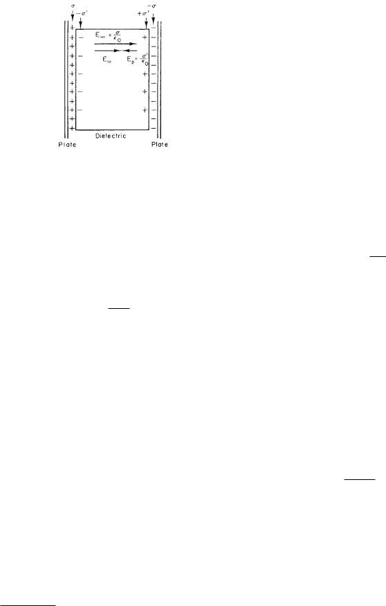
FIGURE 6.17. The polarization electric field reduces the electric field between the plates. The conducting plates could be extracellular and intracellular fluid, and the dielectric could be the cell membrane.

In simple materials all three vectors are parallel and Ep is proportional to Etot. Then we can define the electric susceptibility χ by the equation

Ep = −χEtot.

This can be combined with the previous equation to get

χ

Ep = −1 + χ Eext.

The polarization electric field is thus proportional to both the total electric field (proportionality constant −χ) and the external field [proportionality constant −χ/(1 + χ)]. The former relationship is more fundamental, since the field displacing charges in one atom is the total field, due to both external charges and to the charges in neighboring atoms.

The total field within the dielectric is

The factor κ = 1 + χ is called the dielectric constant of the dielectric. The electric field within the dielectric is reduced by the factor 1/κ from that which would exist without the dielectric. The dielectric constant for typical nerve membranes9 is about 7. The dielectric constant of water is quite high (around 80) because the water molecules can easily reorient their charged ends.

The relationship between the applied field, the polarization field, and the total field can be seen in the following example. The electric field between two parallel sheets of charge of density +σ and −σ per unit area has magnitude Eext = σ/ 0. If there is dielectric between them (such as a cell membrane) and if the polarization in the

9This value is high compared to the dielectric constant for a pure lipid, which is between 2 and 3. See the discussion in Sec. 6.17.

dielectric is uniform, then there is e ectively a charge

±σ induced on the surface of the dielectric that partially neutralizes the external charges. This is shown in

Fig. 6.17. The total electric field within the membrane is

Etot = |Eext + Ep| = σ/ 0 − σ / 0 = σnet / 0 = Eext/κ.

To recapitulate, in Fig. 6.17 Eext is σ/ 0 and depends on the external charge distribution; the potential di erence between the plates depends on the total field, and its magnitude is Etot times the plate separation.

It is customary to refer to two di erent kinds of charge. The free charge is the charge that we bring into a region. We have some control over it. The bound charge is the charge induced in the dielectric by the movement or distortion of atoms and molecules in the dielectric in response to the free charge that has been introduced. Gauss’s law can be written either in terms of the total charge (free plus bound)

or in terms only of the free charge

κEn dS = qfree . (6.21b)

0

The dielectric constant is placed inside the integral sign because the Gaussian surface could pass through materials with di erent values of the dielectric constant.

As another example of the e ect of a dielectric, consider a spherical ion of radius a in which all the charge resides on the surface. In a vacuum, the potential at distance r is v = q/4π 0r, so on the surface of the ion, the potential is q/4π 0a. The work required to bring to the surface an additional charge dq is dW = vdq = qdq/4π 0a. The total work required to place charge Q on the ion is therefore

If the sphere is immersed in a uniform dielectric the total electric field and therefore the potential is reduced by a factor κ. The energy required to assemble the ion is then

This is called the Born charging energy. For an ion of radius 0.2 nm (200 pm) and Q = 1.6 ×10−19 C, the Born charging energy in a vacuum is 5.8 ×10−19 J ion−1. Multiplying by Avogadro’s number gives 3.5 × 105 J mol−1. Often in problems involving charges of a few times the electronic charge, it is convenient to use the energy unit electron volt: 1 eV= 1.6 × 10−19 J. For this problem, the Born charging energy is 3.6 eV ion−1.

If the ion is in a dielectric with κ = 2 (a lipid, for example), the Born charging energy is reduced to 1.8 eV ion−1. Water has a very high dielectric constant (about 80) because the water molecules look roughly like that

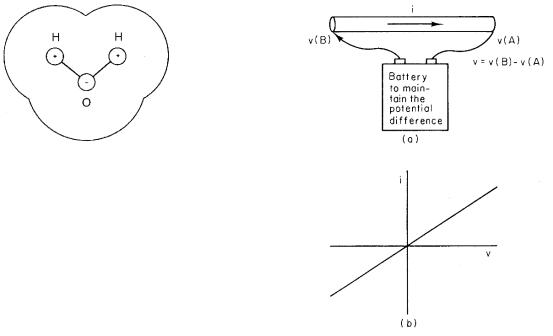
FIGURE 6.18. A schematic diagram of a water molecule. The hydrogen nuclei are 96.5 pm from the oxygen nucleus; the included angle is about 104 ◦. The radius of each hydrogen atom is about 120 pm; the radius of the oxygen atom is about 140 pm. The water molecule has a permanent electric dipole moment.

in Fig. 6.18, and the molecules can easily align with an applied electric field. The same ion in water has a Born charging energy of 0.045 eV. At room temperature, the Boltzmann factor for the energy required to create the ion in vacuum is 3.32 × 10−61. In a lipid, it is 5.76 × 10−31, and in water, it is 0.175. This explains why it is easy to form ionic solutions in water but not in lipids.

6.8 Current and Ohm’s Law

In the electrostatic case, there are no moving charges and no electric field within a conductor. When a current flows in a conductor, charges are moving and there is an electric field.

The electric current i in a wire is the amount of charge per unit time passing a point on the wire. If the amount of charge in time dt is dQ, the current is

The units of the current are C s−1 or amperes (A) (sometimes called amps). The current density j (or jQ in the notation of Chapter 5) is the current per unit area, i/S. The units are C m−2 s−1 or A m−2. In an extended medium, the current density is a vector j at each point in the medium. The direction of j is the direction charge is moving at that point.

If there is no electric field in the conductor, there is no average motion of the charges. (There will be random thermal motion, but it will be equally likely in every direction. This random motion of charges is one cause of “noise” in electrical circuits.) To have a current there must be an electrical field in the conductor; this means that there will be a potential di erence between two points in the conductor. If there is no potential di erence between two points in the conductor, there is no current. For the simple conductor of Fig. 6.19, the current is found to be proportional to the voltage di erence between the ends of the conductor. The current is shown

FIGURE 6.19. A current flows in the wire as long as the battery or some other device maintains a potential di erence between two points on the wire. The potential di erence means that there is an electric field within the wire. If the wire obeys Ohm’s law, the current is proportional to the potential di erence.

flowing from B to A. When v(B) is greater than v(A), v is positive and the current is positive. When v is negative, the current is in the other direction and is also negative.

For the wire of Fig. 6.19, the relationship between current and voltage di erence is linear. In that case, we can write Ohm’s law :

R is called the resistance of the conductor. Since the current is measured in amps and the voltage in volts, its units are V A−1 or ohms (Ω). The reciprocal of the resistance is the conductance G. Its units are Ω−1 or siemens

(S).

Ohm’s law is not universal. It describes only certain types of conductors. Figure 6.20 shows the current– voltage characteristics of several devices that have nonlinear behavior and that make modern electronic circuits possible. They are shown here not for their own sake, but to emphasize the limited validity of Ohm’s law. The nerve cell membrane is not linear.

It is possible to write Ohm’s law in another form. Placing two identical wires in parallel in the circuit of Fig. 6.19 would cause twice as much current to flow (assuming that the battery maintains the voltage di erence at the original level). The current density j remains constant

146 6. Impulses in Nerve and Muscle Cells

FIGURE 6.20. Current–voltage relationships for some nonlinear devices used in electronic circuits. (a) Diode. (b) Transistor. (c) Tunnel diode. (d) Zener diode.

as the cross-sectional area of the wire is changed, when the wire length and voltage di erence are held fixed. Similarly, to maintain the same current through a single wire twice as long requires a voltage di erence twice as great. Therefore, it is voltage per unit length that determines the current. In this spirit, Ohm’s law can be written as

If L is the length of the wire and x the position along it, this can be written as

In three dimensions this alternative statement of Ohm’s law becomes

The σ in this equation10 is the electrical conductivity, measured in (A m−2)/(V m−1) or S m−1. Its reciprocal is the resistivity of the material, ρ. The units of resistivity are Ω m. For a cylindrical conductor, the resistivity and the resistance are related by

ρ1 = SRL

10Note that σ has now been used for two things in this chapter: surface charge per unit area and conductivity. This notation is standard in the literature. You can tell from the context which is meant. Similarly, the symbol ρ is used for charge per unit volume and for resistivity (and for mass density in other chapters). These double usages are found frequently in the literature.

FIGURE 6.21. A resistor connected to a battery.

or

This shows that making the conductor longer increases its resistance, while increasing the cross-sectional area lowers the resistance.

Suppose that an electric field acts on a charge moving in a medium that obeys Ohm’s law. The electric field does work on the charge, but the energy is continually transferred to the medium by collisions between the charge and other particles in the medium. If a charge Q moves to a lower potential, all the energy it gained is transferred to heat. The rate of energy dissipation is the power

The units of power are J s−1 or watts (W). For a material that obeys Ohm’s law, Eq. 6.28 can be combined with Ohm’s law to give

This type of energy loss has clinical significance. If a patient contacts a source of very high voltage such as an 11, 000-V power line, the strong electric fields will cause current to flow throughout the patient’s body or limb, because j = σE. The resistive heating can be enough to boil water within the tissues. If the limb is x rayed, the steam bubbles will look very much like the bubbles that appear in clostridium (gas gangrene) infections; if the x ray is deferred a few days, it will be impossible to tell from the x ray whether the bubbles are due to the electrical injury or subsequent infection.

6.9The Application of Ohm’s Law to Simple Circuits

The ultimate goal of this chapter is to apply Ohm’s law to the axon. Before doing that, however, it is worthwhile to see how it can be applied to some simpler circuits in which the current and voltage are not changing with time.

The simplest circuit is a resistance R connected across a battery, as shown in Fig. 6.21. The battery voltage of