

Intermediate Physics for Medicine and Biology - Russell K. Hobbie & Bradley J. Roth
.pdf9
Electricity and Magnetism at the Cellular Level
This chapter describes a number of topics related to charged membranes and the movement of ions through them. These range from the basics of how the presence of impermeant ions alters the concentration ratios of permeant ions, to the movement of ions under the combined influence of an electric field and di usion, and to simple models for gating in ion channels in cell membranes. It also discusses mechanisms for the detection of weak electric and magnetic fields and the possible effects of weak low-frequency electric and magnetic fields on cells.
Section 9.1 discusses Donnan equilibrium in which the presence of an impermeant ion on one side of a membrane, along with other ions that can pass through, causes a potential di erence to build up across the membrane. This potential di erence exists even though the bulk solution on each side of the membrane is electrically neutral. Section 9.2 examines the Gouy–Chapman model for the charge buildup at each surface of the membrane that gives rise to this potential di erence. This same model is extended in three dimensions to the cloud of counterions surrounding each ion in solution—the Debye–H¨uckel model of Sec. 9.3.
Since water molecules have a net dipole moment, they align themselves so as to nearly cancel the electric field of each ion. Very close to the ion the electric field is so strong that even complete alignment is insu cient to cancel the ion’s field. This saturation of the dielectric is described in Sec. 9.4.
Ions move in solution by di usion if there is a concentration gradient and by drift if there is an applied electric field. The Nernst–Planck equation (Sec. 9.5) describes this motion. When several ion species are moving through a membrane, there can be zero total electric current, even though there is a flow of each species. A constant-field model for this situation leads to the Goldman equations of Sec. 9.6.
The next two sections describe channels in active cell membranes. Section 9.7 describes a simple model for gating—the opening and closing of channels—as well as limitations to the conductance of each channel imposed by di usion to the mouth of the channel. Section 9.8 introduces noise—the fluctuations in channel current that limit measurement accuracy but also can be used to determine properties of the channels.
Section 9.9 describes how channels can detect very small mechanical motions, as in the ear, and how certain fish can detect very small electric fields in sea water. Both of these processes are working near the limit of sensitivity set by random thermal motion.
Section 9.10 introduces an area of great interest and controversy: whether weak, low-frequency electric and magnetic fields can have any e ect on cells. We discuss some of the physical aspects of the problem and conclude that such e ects are highly unlikely.
There are many similarities between the models for biological physics presented in this chapter and the models used in plasma physics [Uehara et al. (2000)].
9.1 Donnan Equilibrium
There is usually an electrical potential di erence across the wall of a capillary. There is also a potential di erence across the cell membrane, and the concentration of certain ion species is di erent in the intracellular and extracellular fluid. In Chapter 3 we saw that if the potential di erence across the membrane is v − v, an ion of valence z is in equilibrium when C /C = e−ze(v −v)/kB T . With this concentration ratio there is no current, even if the membrane is permeable to the species. This result is a special case of the Boltzmann factor, more familiar in
228 9. Electricity and Magnetism at the Cellular Level
[K] |
|
|
[K'] |
|
|
||
[Cl] |
|
|
[Cl'] |
|
|
||
[M+ ] |
|
[M+'] |
|
[M - ] |
|
[M - '] |
|
v = 0 |
|
v' |
|
|
|
|
|
left is 0; on the right it is v . Assume that the concentrations of the large molecules are fixed. The potassium concentration on the left side of the membrane will be assumed known, and we must solve for four variables: K , [Cl], Cl , and v . Therefore, four equations are needed.
The first two equations state that the solutions on either side are electrically neutral:
M+ + [K] = [Cl] + M− , |
(9.1) |
FIGURE 9.1. Ion concentrations on either side of a membrane. Species that can pass through the membrane are indicated by double-headed arrows.
physiology as the Nernst equation (Eq. 3.34):
v − v = − |
kB T |
ln |
C |
RT |
ln |
C |
|||||
|
|
|
|
= − |
|
|
|
. |
|||
ze |
|
C |
zF |
C |
|||||||
It is often said—incorrectly—that the Nernst equation shows how the concentration of an ion species causes the potential di erence across the membrane. We saw in Chapter 6 that the potential di erence across the membrane is caused by layers of charge on each side of the membrane that create an electric field in the membrane. The solutions on each side of the membrane are electrically neutral except at the boundary with the membrane. (If there were an electric field in the solution, ions would move until the field was zero; then Gauss’s law could be used to show that any volume contains zero charge.) We will learn in Sec. 9.2 the typical distance from the membrane occupied by the charged layer, and in Sec. 9.3 we will find the distance scale over which there are microscopic departures from neutrality in a bulk ionic solution.
The concentration di erences do not directly cause the potential di erence. However, if the concentration of an ion species on one side of the membrane is varied, the potential often changes in a manner that is approximated by the Nernst equation over a wide range of concentrations. We will now explore one mechanism by which this can happen. This is particularly important for the walls of capillaries, where charged proteins in the blood are too large to pass through the gaps between cells in the capillary walls, but it is also applicable to the cell membrane.
In Donnan equilibrium, the potential di erence arises because one ion species cannot pass through the membrane at all. Consider the hypothetical case of Fig. 9.1. Permeant potassium ions exist on either side of the membrane in concentrations [K] and K . In this case potassium is the only permeant cation; in a real situation there might be several permeant ions. The membrane is also permeable to chloride ions, which exist in concentrations [Cl] and Cl . Chloride is the only permeant anion. In addition, there are large charged molecules M+ and M−
that cannot pass through the membrane. Their concentrations are M+ , M+ , M− , and M− . For simplic-
ity, we assume they are monovalent. The potential on the
M+ + K = Cl + M− . |
(9.2) |
Equation 9.1 can be solved for [Cl]. It will be convenient to define [M] = M+ − M− and M = M+ − M− :
[Cl] = [K] + ( M+ − M− ) = [K] + [M] . (9.3)
Note that adding any amount of KCl to the solution on the left automatically satisfies this equation, since any increase in [K] is accompanied by a like increase in [Cl].
The other two equations state that the concentrations of potassium and chloride on the two sides of the membrane are related by a Boltzmann factor. Since the valence z = +1 for [K] and −1 for [Cl] we have
|
K |
= |
|
[Cl] |
|
= e−ev /kB T . |
|
(9.4) |
|
|
[K] |
Cl |
|
||||||
|
|
|
|
|
|
||||
The chloride concentration |
on the right |
is |
Cl |
= |
|||||
[Cl] Cl / [Cl] = [Cl] [K] / K , so that from Eq. 9.2K + M = [Cl] [K] / K . This can be rewritten as a quadratic equation in K , since [K] and M are known and [Cl] is calculated from Eq. 9.3:
K 2 + M K − [K] [Cl] = 0.
The solution is |
|
|
|
|
|
|
|
|
|
|
|
|
M |
+ , |
M 2 |
+ 4 [K] [Cl] |
|
K = |
− |
|
|
|
. (9.5) |
|
2 |
|
|||
|
|
|
|
||
(The negative square root is discarded because it would give a negative potassium concentration.) Once we have solved for K , Cl and v are determined from Eq. 9.4. Solutions for di erent values of [K] are shown in Table 9.1 and Figs. 9.2 and 9.3 for the conditions
M+ |
= 145 mmol l−1, |
M+ |
= 15 mmol l−1, |
M− = 30 mmol l−1, |
M− = 156 mmol l−1, |
||
[M] = 115 mmol l−1, |
M = 141 mmol l−1. |
||
|
|
|
− |
The temperature T = 310 K, for which kB T /e = 26.75 mV.
9.2 Potential Change at an Interface: The Gouy–Chapman Model |
229 |
TABLE 9.1. Variation of concentrations and voltage as [K] is varied.
|
|
|
|
[Cl]/[Cl ] = |
|
[K] |
[Cl] |
[K ] |
[Cl ] |
[K ]/[K] |
v (mV) |
0.01 |
115.01 141.01 |
0.01 |
14101 |
−255.57 |
|
0.10 |
115.10 141.08 |
0.08 |
1410.8 |
−193.99 |
|
0.20 |
115.20 141.16 |
0.16 |
705.8 |
−175.46 |
|
0.50 |
115.50 141.41 |
0.41 |
282.8 |
−151.00 |
|
1.00 |
116.00 141.82 |
0.82 |
141.8 |
−132.53 |
|
2.00 |
117.00 142.64 |
1.64 |
71.32 |
−114.15 |
|
5.00 |
120.00 145.13 |
4.13 |
29.03 |
−90.10 |
|
10.00 |
125.00 149.37 |
8.37 |
14.94 |
−72.33 |
|
20.00 |
135.00 158.08 |
17.08 |
7.904 |
−55.30 |
|
50.00 165.00 185.48 |
44.48 |
3.710 |
−35.07 |
||
100.00 215.00 |
233.20 |
92.20 |
2.332 |
−22.65 |
|
200.00 315.00 |
331.21 |
190.21 |
1.656 |
−13.49 |
|
500.00 |
615.00 |
629.49 |
488.49 |
1.259 |
−6.16 |
|
0 |
Curve if [K'] were constant |
|
||
|
-50 |
|
|||
|
|
|
|
|
|
(mV) |
-100 |
|
|
|
|
-150 |
|
|
|
|
|
v' |
|
|
|
|
|
|
|
|
|
|
|
|
-200 |
|
|
|
|
|
-250 |
|
|
|
|
|
0.01 |
0.1 |
1 |
10 |
100 |
|
|
|
[K] (mmole l-1) |
|
|
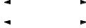
FIGURE 9.3. Membrane potential v vs [K] for the example of Donnan equilibrium. For [K] < 10 mM the curve is like the Nernst equation because [K ] has a nearly constant value of 141 mM. The dashed line shows the relationship if [K ] is constant.
) |
|
|
|
|
|
|
-1 |
600 |
|
|
|
|
|
l |
|
|
|
|
|
|
[Cl'] (mmole |
|
|
|
|
|
|
400 |
|
|
[K'] |
|
|
|
|
|
|
|
|
||
200 |
|
|
[Cl'] |
|
|
|
[K'] or |
|
|
|
|
||
|
|
|
|
|
||
0 |
|
|
|
|
|
|
|
100 |
200 |
300 |
400 |
500 |
|
|
0 |
|||||
|
|
|
[K] (mmole l-1) |
|
|
|
FIGURE 9.2. Variation of [K ] and [Cl ] with [K] in the example of Donnan equilibrium.
Several features of this solution are worth noting. First, changing [K] does change the potential, but the mechanism is indirect. The Boltzmann factor still applies; minuscule changes in concentration are su cient to provide layers of charge on the membrane surface that generate a potential di erence such that these concentrations are at equilibrium. Table 9.1 shows that [K] can vary by three orders of magnitude—from 0.01 to 10, and K changes very little. Therefore, the curve of v vs ln [K] in Fig. 9.3 is nearly a straight line. The dashed line in Fig. 9.3 shows v vs ln [K] if K is held constant. We could equally well have regarded [Cl] as the independent variable.
The impermeable ions enter the equation only as their net charge, [M] = M+ − M− and M = M+ −
M− . As the concentrations [K] and [Cl] get larger, the impermeant ions become less important, the potential approaches zero, and the ratios K / [K] and Cl / [Cl] approach unity.
Donnan equilibrium may well explain the potential that exists across the capillary wall, which is impermeable to negatively charged proteins but is permeable to other ions. There is evidence that it does not adequately explain the potential across a cell membrane. For exam-
ple, the membrane is known to be slightly permeable to sodium, although the sodium concentration is nowhere near what it would be if the sodium were in equilibrium.
9.2Potential Change at an Interface: The Gouy–Chapman Model
In this section we study one model for how ions are distributed at the interface in Donnan equilibrium. The model was used independently by Gouy and by Chapman to study the interface between a metal electrode and an ionic solution. They investigated the potential changes along the x axis perpendicular to a large plane electrode. The same model is used to study the charge distribution in a semiconductor. Biological applications are described by Mauro (1962). We show the features of the model by examining the transition region for the Donnan equilibrium example described in the preceding section.
An infinitely thin membrane at x = 0 is assumed to be permeable to potassium and chloride ions. Their concentrations are K(x) and Cl(x). An impermeant positive cation has concentration M (x) for x > 0. For negative x, M (x) = 0. There are no impermeant anions. Far to the left the potential is zero and the concentrations are [K] and [Cl]. Far to the right they are v , K , Cl , and
M .
The first step is to relate the charge distribution to the potential. If v and E change only in the x direction, then Gauss’s law can be applied to a slab of cross-sectional area S between x and x +dx as shown in Fig. 9.4. The net flux out through the surface at x + dx is Ex(x + dx)S. The net outward flux at x is −Ex(x)S. There is no contribution to the flux through the other surfaces. The total ionic charge in the volume is ρext(x)Sdx. We include the e ect of water polarization by using the dielectric constant for water, which is about κ = 80. Applying Gauss’s law in
230 9. Electricity and Magnetism at the Cellular Level
Ex(x ) |
Ex (x + dx ) |
ρext (x) |
|
x |
x + dx |
(Remember that M (x) = 0 to the left of the origin.) An equivalent general expression is
ρext(r) = e zi [Ci] exp |
−ziev(r) |
|
, |
(9.9b) |
i |
kB T |
|
|
|
|
|
|
|
|
where Ci is the concentration in the region where v = 0. Combining Eqs. 9.7 and 9.9b gives the Poisson–
Boltzmann equation for a dielectric:
FIGURE 9.4. Gauss’s law is applied to the shaded volume to derive Poisson’s equation in one dimension.
the form Eq. 6.21b, we obtain1
Ex(x + dx) − Ex(x) = 4πρext(x) dx , 4π 0 κ
dEx = 4πρext(x) . dx
Finally, since Ex = −∂v/∂x, we have the one-dimensional Poisson equation,
d2v |
= − |
4πρext(x) |
(9.6) |
|
|
|
. |
||
dx2 |
4π 0 κ |
|||
This equation was derived in much the same way that the equation of continuity was combined with Fick’s first law to derive Fick’s second law (Sec. 4.8). The same procedure can be used in three dimensions to derive the general form of Poisson’s equation:
2v = − |
4πρext(r) |
. |
(9.7) |
|
For the model being considered the ions are all univalent, so the ionic charge density at x is related to the concentrations by
ρext(x) = e [K(x) + M (x) − Cl(x)] . |
(9.8a) |
More generally, for a series of ion species each with concentration Ci and valence zi,
ρext(r) = e ziCi(r). |
(9.8b) |
i |
|
The next step is to assume that the concentrations of all ions are given by Boltzmann factors and are therefore related to the potential by
K(x) = |
[K] e−ev(x)/kB T |
for all x, |
|
Cl(x) = |
[Cl] eev(x)/kB T |
for all x, |
(9.9a) |
M (x) = M e−e(v(x)−v )/kB T , x > 0. |
|
||
1Throughout this section we keep 4π in both numerator and denominator that could be canceled. We do this for two reasons. First, the quantity 1/4π 0 has a numerical value of about 9 × 10⁹, which is easy to remember; second, for those who do not use SI units, the factor 1/4π 0 does not appear, but the other factor of 4π remains.
|
4πe |
|
|
ziev(r) |
|
2v = − |
|
zi [Ci] exp |
|
− |
. (9.10) |
4π 0 κ |
|
kB T |
|||
|
|
i |
|
|
|
For the specific problem at hand, the Poisson–Boltzmann equation takes the form
d2v |
= |
|
−4πe |
[K] e−ev(x)/kB T |
− |
[Cl] eev(x)/kB T . |
dx2 |
|
|||||
|
4π 0 κ |
|
||||
This applies for x < 0 only. While it is possible to solve this using numerical techniques [see Mauro (1962)], we will confine ourselves to the case in which ξ = ev/kB T 1 and we can make the approximation eξ ≈ 1 + ξ. (This is accurate to 0.5% for ξ = 0.1, to 10% for ξ = 0.5, and to 25% for ξ = 0.8.) With this approximation
|
|
|
ziev |
|
|
|
|
|
|
|
|
||
ρext = e |
[Ci] zi 1 − |
|
= |
(9.11) |
||
kB T |
||||||
|
|
e2 |
|
2 |
|
|
e |
[Ci] zi − |
|
|
[Ci] zi v. |
(9.12) |
|
kB T |
|
|||||
Far from the membrane the solution is electrically neutral, so the first term vanishes. We are left with the linear Poisson–Boltzmann equation:
4πe2 [Ci] z2
2v(r) = i v(r). (9.13)
The coe cient of v(r) on the right has the dimensions of 1/(length)2. This length will also appear in other contexts. It is known as the Debye length, λD :
|
1 |
= |
4πe2 [Ci] zi2 |
. |
|
(9.14) |
|||||||||
|
λD2 |
|
|
|
|
||||||||||
|
|
|
|
|
4π 0 κ kB T |
|
|||||||||
The linearized Poisson–Boltzmann equation is |
|
||||||||||||||
|
|
|
|
|
2v = |
|
v |
. |
|
(9.15) |
|||||
|
|
|
|
|
|
|
|
||||||||
|
|
|
|
|
λ2 |
||||||||||
|
|
|
|
|
|
|
|
|
|
|
D |
|
|
|
|
For the one-dimensional problem and x < 0, it is |
|
||||||||||||||
|
|
|
|
|
|
d2v |
= |
|
v |
, |
|
|
(9.16) |
||
|
|
|
|
|
dx2 |
λ2 |
|
|
|||||||
|
|
|
|
|
|
|
|
|
|
||||||
|
|
|
|
|
|
|
|
|
|
|
D |
|
|
|
|
where |
|
|
|
|
|
|
|
|
|
|
|
|
|||
|
1 |
|
= |
|
|
4πe2 ([K] + [Cl]) |
. |
(9.17) |
|||||||
λD2 |
|
|
|||||||||||||
|
|
|
|
4π 0κkB T |
|
||||||||||
The methods of Appendix F can be applied to solve this equation.2 The characteristic equation is s2 = 1/λ2D , so
2We have seen this equation before in electrotonus when the membrane capacitance is fully charged (Sec. 6.12).
the solution for x < 0 is v(x) = Ae−x/λD + Bex/λD . The potential is zero far to the left, so A = 0. Therefore, the solution is
v(x) = Bex/λD , x < 0. |
(9.18) |
It is most convenient to write the concentrations for x > 0 in terms of the concentrations far to the right. It is now necessary to include the impermeant ions.
K(x) = K e−e[v(x)−v ]/kB T ,
Cl(x) = |
Cl ee[v(x)−v ]/kB T , |
(9.19) |
M (x) = M e−e[v(x)−v ]/kB T . |
|
|
The linearized Poisson–Boltzmann equation for x > 0 is then
9.3 Ions in Solution: The Debye–H¨uckel Model |
231 |
density |
|
|
v |
|
|
|
|
ρ |
|
||
Potential or charge |
|
|
|
||
-2 |
0 |
2 |
4 |
||
-4 |
x, nm
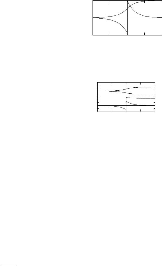
FIGURE 9.5. The potential and charge density in the vicinity of the Donnan membrane. There is a layer of negative charge on the left of the membrane and of positive charge on the right. Each decays with the Debye length given by the ion concentrations far from the membrane.
d2v |
|
|
4πe |
|
|
|
|
K ev(x) |
K ev |
|||||
|
= − |
|
K − |
|
|
|
+ |
|
− Cl |
|||||
dx2 |
4π 0κ |
kB T |
kB T |
|||||||||||
|
|
Cl ev(x) |
Cl ev |
|
|
|||||||||
|
|
|
|
|
|
+ |
|
|
|
|
+ M |
(9.20) |
||
|
− |
kB T |
|
|
|
|
|
|
||||||
|
|
|
|
|
kB T |
|
|
|||||||
|
|
M ev(x) |
|
M ev ! |
|
|
||||||||
|
− |
|
|
|
+ |
|
|
. |
|
|
||||
|
|
kB T |
|
kB T |
|
|
||||||||
Neutrality requires that K + M − Cl = 0. With the definition
1 |
= |
4πe2( K + |
Cl + M ) |
, |
(9.21) |
|||||||
|
λ 2 |
|
|
|
|
|
|
|
|
|||
|
|
|
|
4π 0 κkB T |
|
|
|
|
||||
|
D |
|
|
|
|
|
|
|
|
|
|
|
Eq. 9.20 can be written as |
|
|
|
|
|
|
||||||
|
|
|
|
d2v |
v(x) |
v |
|
|||||
|
|
|
|
|
− |
|
= − |
|
. |
(9.22) |
||
|
|
|
|
dx2 |
λD2 |
λD2 |
||||||
This is an inhomogeneous linear di erential equation with constant coe cients. As pointed out in Appendix F, the most general solution is the sum of the solution to the homogeneous equation (that is, with the right-hand side equal to 0) and any solution of the inhomogeneous equation, with the constants adjusted to satisfy whatever boundary conditions exist. In this case v(x) = v satisfies the inhomogeneous equation, so the most general solution is v(x) = A e−x/λD + B ex/λD + v . Far to the right v = v so B = 0. Therefore, the solution we need is
-1 |
160 |
|
|
|
|
l |
|
|
|
Cl(x) |
|
mmole |
120 |
|
|
|
|
|
|
|
|
||
80 |
|
|
K(x) |
|
|
|
|
|
|
||
Concentration, |
|
|
M(x) |
|
|
|
|
|
|
||
40 |
|
|
K+M-Cl |
|
|
0 |
|
|
|
||
|
|
|
|
||
-40 |
-2 |
0 |
2 |
4 |
|
|
-4 |
x, nm
FIGURE 9.6. Concentration profiles across the Donnan membrane. The concentration K(x)+M (x)−Cl(x) is proportional to the charge density.
Figures 9.5 and 9.6 show the potential, concentration, and charge density for the case [K] = 100 and M = 50 mmol l−1. The other parameters are given in Table 9.2. The value of ev /kB T is 0.23.
Since the radii of ions are about 0.2 nm, the Debye length is several ionic diameters, and the continuous model we have used is reasonable.
The Poisson-Boltzmann equation is widely used to study charged molecules in solution [Honig and Nicholls (1995)]. However, in small-scale systems such as ion channels, which have a size similar to or smaller than the Debye length, continuous models may not be entirely reliable [Moy et al. (2000)].
v(x) = A e−x/λD |
+ v x > 0. |
(9.23) |
This solution for x > 0 must be combined with the solution for x < 0, Eq. 9.18. At x = 0 the potential must be continuous. Therefore B = A + v . Also at x = 0 the electric field, and therefore dv/dx, is continuous. (If dv/dx were not continuous, the second derivative and ρext would be infinite.) This requirement gives the equation B/λD = −A /λD . Solving these two equations, we obtain
A = |
−v λD |
, B = |
v λD |
. |
(9.24) |
λD + λD |
|
||||
|
|
λD + λD |
|
||
9.3Ions in Solution: The Debye–H¨uckel Model
In an ionic solution, ions of opposite charge attract one another. A model of this neutralization was developed by Debye and H¨uckel a few years after Gouy and Chapman developed the model in the previous section. The Debye–H¨uckel model singles out a particular ion and assumes that the average concentration of the counterions surrounding it is given by a Boltzmann factor. Screening

232 9. Electricity and Magnetism at the Cellular Level
TABLE 9.2. Parameters for the Donnan interface when [K] = 100, [M] = 0, and [M ] = 50 mmol l−1 at T = 310 K.
[Cl] |
100 mmol l−1 |
[K]100 mmol l−1
[M] |
0 mmol l−1 |
[K ] |
78.1 mmol l−1 |
[Cl ] |
128.1 mmol l−1 |
[M ] |
50 mmol l−1 |
v |
6.617 mV |
λD |
0.991 nm |
λD |
0.875 nm |
by the counterions causes the potential to fall much more rapidly than 1/r. One major di culty with this assumption is that each counterion is also a central ion; therefore, the notion of a continuous cloud of counterions represents some sort of average.
We consider a situation in which the electric field, potential, and charge distribution are spherically symmetric. We could begin with Eq. 9.7 and look up the Laplacian operator in spherical coordinates. However, it is instructive to derive Poisson’s equation for the spherically symmetric case. Consider two concentric spheres of radius r and radius r +dr. Apply Gauss’s law to the volume contained between the two surfaces. If E is spherically symmetric, the flux through the inner sphere is 4πr2E(r). It points into the sphere and is therefore negative. The outward flux at r + dr is
4π(r + dr)2E(r + dr) |
|
|
|
= 4π r2 + 2rdr + (dr)2 |
E(r) + |
dE |
dr . |
|
|||
|
|
dr |
|
If we keep only terms of order dr or less, the outward flux through the outer sphere is
4πr2E(r) + 8πrE(r)dr + 4πr2 dEdr dr.
The net flux out of the volume is 8πrE(r)dr + 4πr2(dE/dr)dr. The total charge in the shell is ρext(r) times the volume of the shell, 4πr2dr. Therefore, Gauss’s law is
|
|
|
|
|
dE |
|
|
4πr2 |
|
||
8πrE(r)dr + 4πr2 |
|
dr = ρext(r) |
|
dr |
|||||||
dr |
κ 0 |
||||||||||
|
|
|
|
|
|
|
|
|
|||
or |
|
|
|
|
|
|
|||||
|
1 |
|
d |
r2E(r) |
= |
4πρext(r) |
. |
(9.25) |
|||
|
|
|
|
||||||||
|
r2 dr |
|
|
4π 0 κ |
|
||||||
Since E(r) = −dv/dr, the final equation for the potential is
1 d |
r2 |
dv |
= − |
4πρext(r) |
(9.26) |
|||
|
|
|
|
|
. |
|||
r2 dr |
dr |
4π 0 κ |
||||||
The Poisson–Boltzmann equation in spherical coordinates, the analog of Eq. 9.10, is
1 d |
dv |
|
4πe |
|
|
ziev(r) |
||||||
|
|
|
|
r2 |
|
|
= − |
|
zi [Ci] exp |
|
− |
. |
r2 dr |
dr |
4π 0 κ |
|
kB T |
||||||||
(9.27) We again make a linear approximation to the Boltzmann factor to obtain the linear Poisson–Boltzmann equation for spherical symmetry:
1 d |
r2 |
dv |
= |
1 |
v(r). |
(9.28) |
|||
|
|
|
|
|
|||||
r2 dr |
dr |
λ2 |
|||||||
|
|
|
|
||||||
|
|
|
|
|
|
D |
|
|
|
The Debye length λD is defined in Eq. 9.14. With the substitution v(r) = u(r)/r, the equation becomes
d2u |
= |
1 |
u(r), |
(9.29) |
|
dr2 |
λ2 |
||||
|
|
|
|||
|
|
D |
|
|
which is the same as Eq. 9.16. Therefore the solution is
v(r) = |
u(r) |
= |
Ae−r/λD + Ber/λD |
. |
r |
|
|||
|
|
r |
||
Requiring that v(r) approach 0 as r → ∞ means that B = 0. For small r, the electric field (dv/dr) is that of an unshielded ion of charge ze. Therefore A = ze/4π 0 κ, and the final solution is
|
ze |
e−r/λD |
|
||
v(r) = |
|
|
|
. |
(9.30) |
4π 0 κ |
|
||||
|
|
r |
|
||
This is the potential of a point charge ze in a dielectric, modified by an exponential decay over the Debye length. From Eq. 9.14 one sees that the greater the concentration of counterions, the shorter the Debye length.
Table 9.3 shows values of v(r), ξ = ev/kB T , and the potential from an unscreened point charge in water of dielectric constant 80, when the ion concentrations are those given in Fig. 6.3. A typical ion radius is about 0.2 nm. We will discover in the next section that the dielectric constant saturates for r < 0.25 nm. Therefore, values are given in Table 9.3 only for r > 0.3 nm. The table shows that the assumption eξ ≈ 1 + ξ is reasonable only for r > 0.5 nm. The Debye length is λD = 0.77 nm.
The charge density of the ion cloud can be obtained
from Eqs. 9.26 and 9.30. The result is |
|
|||
ρext(r) = |
−ze |
|
e−r/λD . |
(9.31) |
4πλ2 |
|
|||
|
r |
|
||
|
D |
|
|
|
The total charge in the counterion cloud inside a sphere
of radius a is
a
4πr2ρext(r) dr.
0
Adding to this a point charge ze at the origin gives the total charge due to both the ion and the counterion cloud inside radius a:
q(a) = ze 1 + |
a |
e−a/λD . |
(9.32) |
|
|||
|
λD |
|
|
9.4 Saturation of the Dielectric |
233 |
TABLE 9.3. The Debye-H¨uckel potential for a monovalent ion in a solution of ions at the concentration given in Fig. 6.2 for the interior of an axon. Also shown are the parameter zev/kB T , the unscreened potential, and the charge inside a sphere of radius r.
r (nm) |
v(r) (mV) |
e/(4π 0 κr) (mV) |
ev/kB T q(r)/e |
|
0.3 |
40.6 |
59.9 |
1.52 |
0.94 |
0.4 |
26.8 |
44.9 |
1.00 |
0.90 |
0.5 |
18.8 |
36.0 |
0.70 |
0.86 |
0.6 |
13.8 |
30.0 |
0.51 |
0.82 |
0.7 |
10.4 |
25.7 |
0.39 |
0.77 |
0.8 |
8.0 |
22.5 |
0.30 |
0.72 |
0.9 |
6.2 |
20.0 |
0.23 |
0.67 |
1.0 |
4.9 |
18.0 |
0.18 |
0.63 |
1.2 |
3.2 |
15.0 |
0.12 |
0.54 |
1.4 |
2.1 |
12.8 |
0.08 |
0.46 |
1.6 |
1.4 |
11.2 |
0.05 |
0.39 |
1.8 |
1.0 |
10.0 |
0.04 |
0.32 |
2.0 |
0.7 |
8.99 |
0.03 |
0.27 |
2.2 |
0.5 |
8.17 |
0.02 |
0.22 |
2.4 |
0.3 |
7.49 |
0.01 |
0.18 |
2.6 |
0.2 |
6.91 |
0.01 |
0.15 |
2.8 |
0.2 |
6.42 |
0.01 |
0.12 |
3.0 |
0.1 |
5.99 |
0.00 |
0.10 |
|
|
|
|
|
This function approaches ze, the charge of the point ion, as a → 0, and it approaches 0 as a → ∞. Table 9.3 also shows the values of q(a)/e. Ninety percent of the counterion charge resides within 3 nm of the central ion. The charge on the central ion is half neutralized by charge in a sphere of radius 1.3 nm, about six ionic radii.
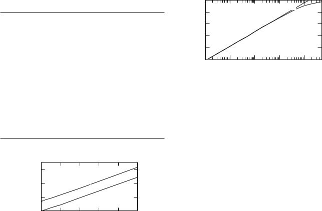
Figure 9.7 shows schematically an ion of radius 0.2 nm. Since a monovalent ion will be neutralized by a single counterion, it is clear that the assumption of a continuous charge distribution equal to the average is a bit strained. The shaded circle of radius 0.25 nm represents the region in which the water molecules are completely polarized and the dielectric constant is less than 80; this is discussed in the next section. (We have ignored the fact that close to the central ion the linear approximation is not valid.)
9.4 Saturation of the Dielectric
The electric field in a vacuum at distance r from a point charge q is E = q/(4π 0r2). If the charge is in a dielectric, the field is reduced by a factor 1/κ, except at very small distances, where the electric field is so strong that the polarization of the dielectric is saturated.
A molecule of water appears schematically as shown in Fig. 6.18. The radius of each hydrogen atom is about 0.12 nm; the radius of the oxygen is about 0.14 nm. Each hydrogen nucleus is 96.5 pm from the oxygen; the angle between them is 104 ◦. The hydrogen atoms share their electrons with the oxygen in such a way that each hydro-
FIGURE 9.7. Schematic picture of the regions surrounding an ion. The solid circle in the center represents the ion of radius 0.2 nm. The shaded circle shows the region in which the polarization of the water is saturated. The outer circle of radius 1.3 nm represents the region within which the cloud of counterions has neutralized half of the charge on the ion, which means that on the average a counterion will be in this region half of the time. This radius depends on the ion concentrations that are those for the interior of a squid axon. A scale drawing of a water molecule is also shown.
gen atom has a net positive charge and the oxygen has a net negative charge. A pair of charges ±q separated by distance b has an electric dipole moment pe of magnitude pe = qb. The vector points from the negative to the positive charge. The magnitude of the dipole moment of a water molecule is 6.237 × 10⁻³⁰ C m.
Each molecule of a dielectric in an applied electric field has an induced dipole moment that reduces the field. This dipole moment can be caused by a displacement of the electron cloud with respect to the nucleus, or it can represent (as for a polar molecule like water) an average molecular alignment against the tendency of thermal motion to orient the water molecules randomly.
The average induced dipole moment gives rise to the polarization field Epol [Eqs. 6.19–6.20]. To see the relationship, consider a small volume in the dielectric with N molecules per unit volume. Each molecule has a dipole moment pe = qb. Far from this volume, the potential is due primarily to the dipole moment of each molecule. This can be shown by arguments like those in Secs. 7.3 and 7.4. The potential depends on the total dipole moment of the volume. The total number of dipoles in the volume is N Sdx, so ptot = peN Sdx. This is equivalent to a charge q = peN S on the ends of the volume element, or a surface of charge density
σ |
= |
q |
= p |
N. |
(9.33) |
|
|||||
q |
|
S |
e |
|
|
|
|
|
|
|
Now consider a parallel-plate capacitor as shown in Fig. 9.8. Imagine a series of small volume elements in the dielectric. The induced charges ±σq on adjacent surfaces of each row of volume elements cancel except at the end of each row. The polarization field is therefore due entirely to the induced charge of surface density ±σq at each end of the dielectric. The magnitude of the field is
|
σ |
|
N pe |
|
|
||
Epol = |
|
q |
= |
. |
(9.34) |
||
0 |
0 |
||||||
|
|
|
|
||||
234 9. Electricity and Magnetism at the Cellular Level
|
|
|
E ext |
|
+σ |
−σ' |
p tot |
+σ ' |
−σ |
|
E pol
FIGURE 9.8. A dielectric is placed in a parallel-plate capacitor that has charge ±σ on each plate. A dipole moment of magnitude ptot is induced in each volume element of the dielectric. The total e ect is the same as a charge density ±σ induced on the surfaces of the dielectric.
The quantity N pe is the dipole moment per unit volume and is called the polarization P .
As the external electric field is increased, Epol, which points in the opposite direction, also increases. This corresponds to the water molecules becoming more and more aligned. From the definition of susceptibility and the dielectric constant in Sec. 6.7, the magnitudes are related by
|Epol| = |
χ |
|
|
1 |
|
|
|
|Eext| = |
1 − |
|
|
|Eext| . |
|
1 + χ |
κ |
|||||
For a monovalent ion in water, Epol = (79/80)Eext = (79/80)e/(4π 0r2). When the dipoles are completely aligned, Epol saturates at its maximum value, given by Eq. 9.34 with the molecular dipole moment substituted for pe. The number of water molecules per unit volume is obtained from the fact that 1 mol has a mass of 18 g, occupies 1 cm3 g−1, and contains NA molecules:
-1 |
1.6 |
|
|
|
|
V m |
|
|
|
||
|
|
|
|
||
11 |
1.2 |
|
|
|
|
of 10 |
|
|
|
||
0.8 |
Eext |
|
|
||
in unit |
0.4 |
Epol |
|
|
|
field |
|
|
|||
0.0 |
|
|
|
||
E |
0.2 |
0.3 |
0.4 |
||
0.1 |
|||||
|
r, nm
FIGURE 9.9. The electric field around a monovalent point charge and the polarization electric field due to the water. The polarization field saturates for r < 0.23 nm.
gradual transition of the dielectric constant from 80 to 1.3
Close to an ion the potential is larger than q/(4π 0 κ r). This changes the Born charging energy [Eq. 6.22] and the free energy change as an ion dissolves in a solvent [Bockris and Reddy (1970), Chapter 2]. Also, close to an ion the continuum approximation breaks down.
9.5Ion Movement in Solution: The Nernst–Planck Equation
Solute particles can move by di usion. They can also move if they have an average velocity Vsolute. There are two ways they can acquire an average velocity. The first is if they are at rest on average with respect to a moving solution. This is called solvent drag. The second is for the solute particles to be dragged through the solution by an external force that acts on them, such as gravity or an electric force, balanced by the viscous force on the particles. In both cases, the number per unit area per unit time crossing a plane is CVsolute. The solute particle fluence rate (particle current density) due to both di usion and the solute velocity in the x direction is4 (Sec. 4.12)
dC
js = −D dx + CVsolute. (9.35)
Epol(max)
=
(NA molecule/mol)(1 g/cm3)(106 cm3/m3)
(18 g/mol) 0 C V−1 m−1
×6.237 × 10−30 C m/molecule
=2.36 × 10¹⁰ V m−1.
|
Suppose that an external force F = zeE acts on the |
|
solute particles in the x direction. They will be acceler- |
|
ated until the viscous drag on them is equal to the magni- |
|
tude of F . But we saw in Chapter 4 that the viscous drag |
|
is f = −β(Vsolute − Vsolvent) where Vsolute − Vsolvent is the |
|
relative velocity of the solute through the solvent. Coe - |
|
cient β is related to the di usion constant by β = kB T /D. |
Figure 9.9 shows the fields Eext and Epol around a monovalent ion. As Epol saturates, Etot rises toward the value it would have without a dielectric. The dielectric constant falls from 80 to 1 at about 0.23 nm. A more accurate model predicts similar behavior, but with a more
3A more sophisticated model for the alignment of the electric dipoles in the electric field is analogous to that for magnetic moments in Sec. 18.3.
4We use x for the distance in the direction parallel to E because z is used for valence.

9.5 Ion Movement in Solution: The Nernst–Planck Equation |
235 |
Therefore, the particles are no longer accelerated when
Vsolute − Vsolvent = zeE/β. |
(9.36) |
Equation 9.35 can be rewritten as
dC
js = −D dx + C [Vsolvent + (Vsolute − Vsolvent)] .
Now Vsolvent is the volume of solvent that flows per unit area per unit time and is just jv . With this substitution and using Eq. 9.36, the particle current density is
js = −D |
dC |
+ Cjv + CzeE |
D |
(9.37) |
|
|
|
. |
|||
dx |
kB T |
||||
The first term represents solute motion due to di usion, the second represents solute dragged along with the bulk flow of the solution (solvent drag), and the third represents drift due to the applied electric field.
We will consider only the case in which there is no bulk flow of solution, so jv = 0. The equation then reduces to the Nernst–Planck equation:
js = −D |
dC |
+ |
zeE |
(9.38) |
|
|
|
DC. |
|||
dx |
kB T |
||||
Di usion is always toward the region of lower concentration, while for positive charge the Vsolute term is in the direction of E. For negative charges it is in the opposite direction.
Consider the current density in bulk solution between planes at x = 0 where v(x) = 0 and x = L where v(x) = v. If there is no concentration gradient and the potential changes uniformly, then E = −dv/dx = −v/L points in the −x direction, and the particle current density is js = −zeDCv/kB T L. The electrical current density j is obtained by multiplying js by the charge on each particle, ze:
j = − |
z2e2DCS v |
= − |
G(C) |
v. |
(9.39) |
||
|
|
|
|
||||
kB T L S |
S |
||||||
If v(L) > v(0), the current is to the left and is negative. Recalling that G = σS/L = 1/R = S/ρL, we obtain the conductivity in bulk solution
σ = |
1 |
= |
z2e2DC |
. |
(9.40) |
|
|
|
|
||||
|
ρ |
|
kB T |
|
||
If several ion species carry current and can be assumed to move independently, then the total conductivity is the sum of the conductivities for each ion. Table 9.4 shows contributions to the conductivity for various species at typical concentrations.
This model is satisfactory for material such as the inside of an axon where the concentrations are constant and the material is electrically neutral, so that the ions themselves do not on average contribute to the electric field. We have assumed that the ions move independently, which will happen only if the electric field of other ions can be ignored.
TABLE 9.4. Conductivities of ions at various concentrations at 25◦C, calculated using Eq. 9.40. Di usion constants for each ion are from Hille (2001, p. 317). Concentrations are typical of mammalian nerve and are from Hille (2001, p. 17). The conductivities of each species add, and ρ = 1/σ. Larger ions with very small di usion constants make the solutions electrically neutral.
|
D (m2 s−1) |
C (mmol l−1) |
σ (S m−1) |
ρ (Ω m) |
|
Extracellular squid axon |
|
||
Na |
1.33 × 10⁻⁹ |
143 |
0.723 |
|
K |
1.96 × 10⁻⁹ |
4 |
0.029 |
|
Cl |
2.03 × 10⁻⁹ |
123 |
0.936 |
0.592 |
|
|
|
1.688 |
|
|
Intracellular squid axon |
|
||
Na |
1.33 × 10⁻⁹ |
12 |
0.060 |
|
K |
1.96 × 10⁻⁹ |
155 |
1.139 |
|
Cl |
2.03 × 10⁻⁹ |
4.2 |
0.032 |
0.812 |
|
|
|
1.231 |
|
|
|
|
|
|
We can model ions flowing from a region of one concentration to another (such as crossing the axon membrane) with the Nernst–Planck equation. Writing it for the electric current density and using the fact that E(x) = −dv/dx, we have
j = −zeD |
dC |
− |
z2e2D dv |
(9.41) |
|||
|
|
|
|
C. |
|||
dx |
kB T |
dx |
|||||
It is simpler to use the dimensionless variable u(x) = zev(x)/kB T , which is the ratio of an ion’s energy to thermal energy:
|
|
dC |
|
|
||
|
|
du |
|
|||
j = −zeD |
|
|
+ C |
|
. |
(9.42) |
|
dx |
dx |
||||
If we assume that dv/dx is constant throughout the region, v(0) = 0 and v(L) = v, then the gradient is dv/dx = v/L, and Eq. 9.41 becomes
dC |
− |
1 |
C = − |
j |
, |
(9.43) |
dx |
λ |
zeD |
where the characteristic length for this model (not the Debye length) is
λ = |
L |
= |
kB T L |
. |
(9.44) |
u |
|
||||
|
|
zev |
|
||
Equation 9.43 is the same as Eq. 4.58, except for the denominator of the term involving j. Here the denominator is zeD because j is the electric current density instead of the particle current density. The solution analogous to Eq. 4.62 is
j = |
zeD |
C0eL/λ − C0 |
= |
zeD |
C0e−u − C0 |
, (9.45) |
|
λ eL/λ − 1 |
λ e−u − 1 |
||||||
|
|
|
|||||
where C0 is the ion concentration at x = 0 and C0 is the concentration at x = L.

236 9. Electricity and Magnetism at the Cellular Level
units) |
Nernst-Planck |
|
|
|
, (arbitrary |
Tangent |
|
|
|
Line |
|
|
|
|
|
|
|
|
|
Na |
|
|
|
|
j |
|
|
|
|
-200 |
-100 |
0 |
100 |
200 |
|
v |
(mV) |
|
|
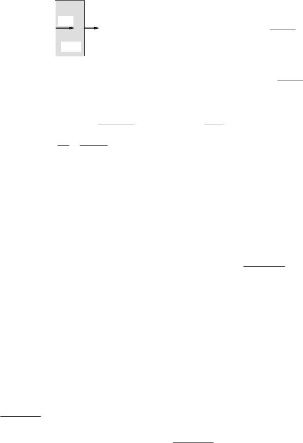
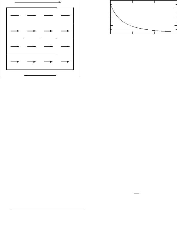
FIGURE 9.10. Sodium current versus applied potential for the constant field Nernst–Planck model when the sodium concentration is 145 mM on the left and 15 mM on the right. The calculation was done using Eq. 9.46 for T = 293 K. The tangent line was calculated using Eq. 9.48. The nonlinearity or rectification occurs because of the di erent ion concentrations on each side.
This equation was used to derive the tangent line shown in Fig. 9.10.
The constant-field model is an oversimplification. The field can be distorted by fixed charges near the channel through which the ions are flowing. Moreover, the model is internally inconsistent. There are electric fields generated by the flowing ions, which become important at high concentrations. The fact that j = 0 when the potential is equal to the Nernst potential is fundamental and holds for any ion or model for conduction. It can be derived in the general case from Eq. 9.43 (see the Problems). A self-consistent analytic solution for the case of a single ion species has been known for 50 years. The solution has been extended by many workers and has been generalized by Leuchtag and Swihart (1977) to the case in which all the ions have the same charge.
The current vanishes if C0eL/λ − C0 = 0, or C0/C0 = eL/λ = e−zev/kB T = e−u. This is the Boltzmann factor.
Equation 9.45 can be written in terms of the original variables:
j = −z2e2Dv C0e−zev/kB T − C0 = −zeDu C0e−u − C0 .
kB T L e−zev/kB T − 1 L e−u − 1
(9.46) It is interesting to compare this to Eq. 9.39. Since G depends on concentration, it is useful to factor out a factor C0 and write
j = |
− |
z2e2DC0 e−zev/kB T − C0/C0 v |
|
||||||
|
kB T L |
|
e−zev/kB T − 1 |
|
|
||||
= |
− |
G(C0) |
|
e−zev/kB T − C0/C0 |
v. |
(9.47) |
|||
|
|
||||||||
|
S |
e−zev/kB T − 1 |
|
||||||
If C0 = C0, we recover Eq. 9.39. Figure 9.10 shows the current density in A m−2 for a situation where C0 = 145 mmol l−1and C0 = 15. The di usion constant for sodium from Table 9.4 has been used. Because C0 > C0, equilibrium occurs when v = +57.3 mV at 20 ◦C.
Note the nonlinearity of the current–voltage relationship that arises because C0 =C0. For very negative potentials the flow is almost entirely from left to right and the current density approaches G(C0)v/S while for very positive potentials the flow is from right to left and the current density approaches G(C0)v/S. This asymmetry is fundamental. It occurs because there are di erent numbers of charge carriers on the left and right. When this behavior is seen in channels in cell membranes, they are often called rectifier channels. This same asymmetry in di erences in the concentration of charge carriers is responsible for rectification in semiconductors.
Near the Nernst potential the current density has the form j = −(G/S)(v − vNernst) if
G |
= |
G(C0)(zevNernst/kB T ) |
(9.48) |
||
|
|
|
. |
||
S |
S ezevNernst/kB T − 1 |
||||
9.6Zero Total Current in a Constant-Field Membrane: The Goldman Equations
The Nernst-Planck equation can be used to calculate the current due to movement of ions through a membrane in which there is a constant electric field. We assume a constant field because it leads to an analytic solution and because we have no knowledge of internal structure or the behavior of counterions which could change the field. The resulting equations are called the Goldman or the
Goldman–Hodgkin–Katz (GHK) equations.
The GHK equations can be derived by assuming either a homogeneous membrane, in which case the Nernst– Planck equation is simply applied to each species, or cylindrical pores of constant cross section. Since we know that the pores do not have a constant electric field (Sec. 9.7) and it is quite unlikely that they have constant cross section, the GHK equations are an approximation. Nevertheless, they has been used widely in the study of excitable membranes.
We will show the derivation for a cylindrical pore that has a constant circular cross section. We use cylindrical coordinates (r, φ, x), where x is the axis of the cylinder. (Again, z denotes the valence of the ions.) Let the outside of the membrane be at x = 0 and the inside at x = L, where the potential is v and u = zev/kB T . The arguments of Sec. 5.9 about the r and x dependence can be applied to Eq. 9.42. The analog of Eq. 5.37 is
|
∂C(r, x) |
|
u |
|
|
j(r) = −zeD(r, a, Rp) |
|
+ |
|
C(r, x) |
. (9.49) |
∂x |
L |
||||
Again the concentration can be written as C(r, x) =
C(x)Γ(r). Equation 9.49 becomes |
|
|
|
|
|
|
∂C(x) |
|
u |
|
|
j(r) = −zeΓ(r)D(r, a, Rp) |
|
+ |
|
C(x) |
. (9.50) |
∂x |
L |
||||