Intermediate Physics for Medicine and Biology - Russell K. Hobbie & Bradley J. Roth

5.16 for di erent values of ∆Z/λ, the ratio of the pore length to the e ective di usion distance.

These curves determine the shape of the concentration profile along the pore. If the flow is zero, λ = De /jv (1 − σ) is infinite and ∆Z/λ is zero. We then have pure di usion, and the concentration changes uniformly along the pore, corresponding to the straight line in Fig. 5.16. The plots in Fig. 5.17 show what the concentration profiles are like for di usion to the left and to the right when the flow is to the right. Compare the shape of the concentration profile on the left in Fig. 5.17 with the curve for ∆Z/λ = 1 in Fig. 5.16. When the concentration is higher on the left, we have to take the mirror

a pore for di usion to the left and di usion to the right. The fluid on each side of the pore is well stirred and of su cient volume so that concentrations do not change with time.

image of Fig. 5.16; the curve for ∆Z/λ = −1 gives the concentration profile in Fig. 5.17 on the right.

As the pore becomes very long compared to the diffusion length (for example, |∆Z/λ| = 10 or more), the concentration along the pore is nearly that carried into the pore by bulk flow from the left until we get to the far end, where di usion back up the pore gives a smooth transition to the final concentration on the right.

pd(z) = pdw (z) + (1 − σ)kB T C(z).

This is consistent with the solvent drag flux at position z in the pore, which was given in Eq. 5.45a by

jv f C(z) = jv (1 − σ)C(z).

The “e ective” concentration for solvent drag is (1 − σ)C(z).

5.9.3 Summary

To summarize, the combination of solvent and a solute with reflection coe cient has a volume flux

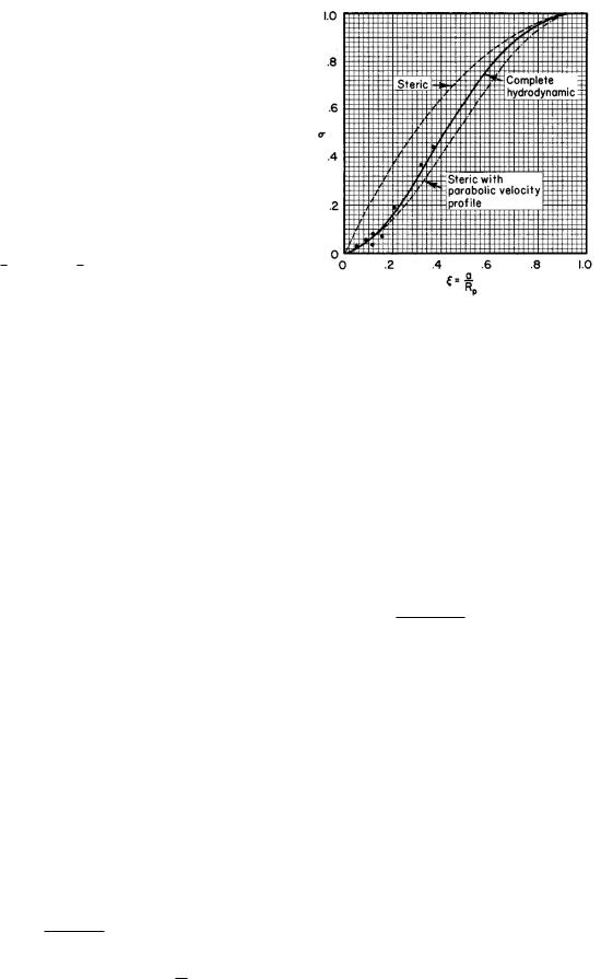
FIGURE 5.18. Calculated values of the reflection coe cient are indicated by the lines. Calculations are shown for the simple steric factor, the steric factor weighted by a parabolic velocity profile, Eq. 5.60, and a more detailed calculation, which takes account of the distortion of the velocity profile by the solute particles. The data points are from Durbin (1960) as reinterpreted by Bean (1972).

and a solute flux

The hydraulic permeability is

5.9.4 Reflection Coe cient

We have referred previously to the fact that the centers of solute particles can occupy only a fraction of the pore volume. A solute particle’s center cannot be further from the pore axis than Rp − a. The simplest correction is the steric factor, seen on p. 120. The ratio of e ective area to total area approximates 1 − σ. If ξ = a/Rp, then

where G(x) is given by Eq. 5.50b. The parameter x is

Notice that the solvent drag term as well as the di usion term depends on ∆Cs, through the factor Cs.

σ = 2ξ − ξ2.

A better calculation was seen in the preceding subsection. Accept the fact (quoted from thermodynamic results) that the same σ occurs in the equations for Jv and Js. We saw that the edges of the pore have less bulk flow than the center, so that the steric e ect overestimates how many particles are reflected. From Eq. 5.44b,

These two approximations to σ are plotted in Fig. 5.18. It was mentioned in a footnote that the calculation which resulted in Eq. 5.44a neglected the change in velocity profile caused by the solute particles. More rigorous calculations have been done by Levitt (1975) and by Bean

(1972, pp. 29–35). Levitt’s result is

This is valid for ξ < 0.6. The three equations for σ are plotted in Fig. 5.18, along with some experimental data

128 5. Transport Through Neutral Membranes

F1

FIGURE 5.19. Plot of ω/ω0 for experimental data by Beck and Schultz (1970) and a calculation by Bean (1972).

from Durbin (1960) using the pore radius assigned by Bean.

FIGURE 5.20. The forces on a membrane with pores. The fluid on the left exerts force F1 due to the hydrostatic pressure p. A similar force F1 is exerted on the right. Solute molecules like A are reflected at the pore edge and exert force F2. Solute molecule B enters the pore. It contributes to the viscous force of the flowing fluid on the cylindrical walls of the pore, F3. F3 is to the right if the fluid flows from left to right through the pore.

5.9.5 The E ect of Pore Walls on Di usion

The solute permeability is given by

ωRT = nπRp2De .

∆Z

The e ective di usion coe cient takes into account the steric factor as well as the drag on the solute particles by the pore walls. If the pore had an infinitely large diameter, the unrestricted permeability would be

where D is the di usion coe cient for an infinite medium. Figure 5.19 shows some data from Beck and Schultz (1970) and a curve for ω/ω0 calculated by Bean (1972).15 In Europe, filtration rather than dialysis is used to treat kidney patients. There is evidence that some as yet unidentified toxin of medium molecular weight accumulates in the blood. Comparison of 1 − σ from Fig. 5.18 with ω/ω0 from Fig. 5.19 shows that solvent drag removes medium-sized molecules more e ectively. The fluid

and electrolytes lost by the patient must be replaced.

5.9.6 Net Force on the Membrane

We conclude the section by calculating the force of the fluid on the membrane. The results give some insight into the nature of osmotic pressure.

15The steric factor, which Bean includes separately, is built into De through the function Γ(r).

A membrane of total area S is pierced by n pores per unit area of radius Rp. The pressures in the fluid on each side of the membrane are p and p . A solute with reflection coe cient σ has concentration C on the left and C on the right. We want to calculate the total force exerted by the fluid on the membrane. There are three contributions to this force. These can be understood by referring to Fig. 5.20.

Forces F1 and F1 are the forces exerted by the fluid on the walls of the membrane on each side. They are obtained by multiplying the total pressure on each side by the area of the membrane that is not occupied by pores. In a total area S there are nS pores, each of area

πRp2.

F1 = pS 1 − nπRp2

F1 = p S 1 − nπRp2 .

Forces F2 and F2 are exerted by solute molecules reflected from the pore region, such as molecule A in Fig. 5.20. These are the ones that contribute to the osmotic pressure. The net force to the right is therefore the total pore area SnπRp2 times the impermeant part of the osmotic pressure di erence:

Force F3 is the viscous drag exerted on the walls of the pores by the water and permeant solute molecules flowing

through them. To calculate it we recall that the viscous force per unit area is −η (∂v/∂r) . The velocity is v = jv . Di erentiating Eq. 5.43,we obtain

∂jv = − 1 ∆ (p − σπ) 2r. ∂r 4η ∆Z

The total force is η times this quantity evaluated at r = Rp, times total area of the cylindrical walls of all the pores, which is (Sn) (2πRp∆Z) :

The net force on the membrane is the sum of these forces:

We see that the net force on the membrane is the total pressure di erence times the total area of the membrane, regardless of the di erences in osmotic pressure on each side. Both solute and solvent exert a force on the nonpore area of the membrane. The solute molecules at the membrane surface whose centers are within the area of a pore may be reflected or may enter the pore. If they are reflected, they contribute to the force when they strike the membrane at the edge of a pore. If they are not reflected, they enter the pore and contribute to the viscous drag on the membrane due to flow through the pore.

Symbols Used in Chapter 5

fTemporary function

nNumber of moles

131up of two main components: albumin (molecular weight 75,000) 4.5 g per 100 ml and globulin (molecular weight

130 5. Transport Through Neutral Membranes

Section 5.4

Problem 4 When a person is given an intravenous fluid, the solute concentration in the fluid must be matched to the solute concentration in the blood to avoid problems arising from a change in the blood’s osmotic pressure. One such fluid, called “isotonic saline,” can be made by adding salt (NaCl) to distilled water. The osmolarity of the blood is about 0.3 osmole.

(a)How many grams of NaCl must be added to a liter of water to make isotonic saline? What fraction of the

solution’s mass is NaCl? (Hint: Recall that NaCl dissolves into Na+ and Cl−, and both contribute to the osmotic pressure.)

(b)Repeat for dextrose, C6H12O6, which does not dissociate.

Problem 5 An understanding of osmotic pressure is important in medicine. Consider the case reported by Steinmuller (1998) in the New England Journal of Medicine. A 5% solution of albumin was needed to infuse into a patient with kidney disease (renal insu ciency). No 5% solution was available, so the hospital pharmacy used 25% albumin diluted 1:4 with pure water. Injection of the solution into the patient caused renal failure. The albumin in a 25% albumin solution has an osmolarity of about 36 mosmol. Typically, such a solution also contains about 300 mosmol of other ions (see Problem 4).

(a)Calculate the osmolarity of the solution injected into the patient.

(b)Calculate the osmolarity of the solution if the pharmacy had properly used isotonic saline instead of pure water to perform the 1:4 dilution.

Problem 6 Articular cartilage covers the ends of bones in joints and allows the bones to move smoothly against each other. It contains a network of collagen fibers that can exert a mechanical tensile stress to resist tissue swelling, resulting in a pressure Pc within the cartilage. The collagen fibers do not withstand compression. The cartilage also contains proteoglycan molecules that cause tissue swelling because of their osmotic pressure, πPG. One can determine Pc by placing the cartilage in a polyethylene glycol solution with osmotic pressure πPEG, measuring πPG and πPEG, and using the relationship Pc =

πPG − πPEG.

(a)What is the excess pressure Pc exerted by the collagen matrix under normal conditions (πPEG = 0)?

(b)At what value of πPEG does the collagen matrix exert no tensile stress (become “limp”)?

(c)Plot Pc vs. πPEG. Find a linear equation that fits the data.

(d)Osteoarthritis is thought to occur when the collagen matrix is weakened. If the collagen in an arthritic joint

can only exert a pressure of 2 atm when πPEG = 0, by how much will the tissue swell (by what percent will its volume change?)

In (b) and (d), assume that only the proteoglycans cause osmotic pressure and that their number does not change, but the tissue volume increases as the tissue swells with water. This problem is based on the work of Basser et al. (1998), but the data have been modified.

Section 5.5

Problem 7 Suppose that Lp is expressed in m3 N−1 s−1 or m s−1 Pa−1. Find conversion factors to express it in

(a)ml min−1 cm−2 torr−1.

(b)ml s−1 cm−2 (in. water)−1.

(c)ml s−1 cm−2 (lb in.−2)−1.

Problem 8 An ideal semipermeable membrane is set up as shown. The membrane surface area is S; the crosssectional area of the manometer tube is s. At t = 0, the height of fluid in the manometer is zero. The density of fluid is ρ. Show that the fluid height rises to a final value with an exponential behavior. Find the final value and the time constant. Ignore dilution of the solute.

PEG

fluid

cartilage collagen

PG bone

Problem 9 Consider the design of a lecture demonstration apparatus to show osmotic pressure that uses a commercially available filter as shown in the drawing. Assuming well-stirred fluid on both sides of the membrane

and neglecting the change of solute concentration in the manometer tube as water flows in, one finds that height z increases to the equilibrium value exponentially, with a time constant obtained in the previous problem. What would be the time constant if one used the membrane described in Fig. 5.10? For that membrane Lp =1 ml min−1 m−2 torr−1, and the total membrane area is S = 0.2 m2. Suppose that the inner radius of the manometer tube is 1 mm. (One could not use sucrose as a solute, because this particular membrane is permeable to molecules of molecular weight less than 50,000.)

Problem 10 A cell has variable volume V and fixed surface area S. The total hydrostatic pressure p is the same inside and outside the cell, and there is complete and instantaneous mixing. Initially the interior and exterior are both pure water. The initial volume of the cell is V0. At t = 0, the exterior is bathed in a solution containing an impermeant solute of concentration C0.

(a)Does the cell shrink to zero volume or expand to its maximum volume, which is a sphere of surface area S?

(b)Derive a di erential equation for the volume change and integrate it to find how long it takes for the cell to reach zero or maximum volume.

Problem 11 A cell has variable volume V and fixed surface area S. The total hydrostatic pressure p is always the same both inside and outside the cell. There is complete and instantaneous mixing both inside and out. An impermeant solute has an initial concentration C(0) both inside and outside. The initial cell volume is V0. At t = 0 the exterior solute is removed.

(a)Does the cell shrink to zero volume or expand to its maximum volume, which is a sphere of surface area S?

(b)Derive a di erential equation for V (t) and find how long it takes for the cell to reach zero or maximum volume.

Section 5.6

Problem 12 Two membranes have permeabilities ω1RT and ω2RT . Find the permeability of a two-layered membrane in terms of ω1 and ω2.

Problem 13 Solute is carried through a pipe by solvent drag. The radius of the pipe is b. The average flow along

Problems 131

the pipe is jv (independent of r because it has been averaged over r). Assume that within the pipe the concentration of solute is independent of radius and can be written as C(z). The solute is carried along purely by solvent drag. Solute concentration outside the pipe is zero. Solute di uses through the wall of the pipe, which has solute permeability ωRT . In terms of jv , b, and ωRT , obtain a di erential equation for C(z) and show that C decays exponentially along the pipe. Find the decay constant.

Section 5.7

Problem 14 A kidney machine has a membrane permeability ωRT = 0.5 × 10−3 cm s−1. If the membrane area is 1 m2, the volume of body fluid is 40 l, and the volume of dialysant is e ectively infinite, what is the time constant? How long will it take to reduce the BUN (blood urea nitrogen) concentration from 120 mg per 100 ml to 20 mg per 100 ml?

Problem 15 Find the pair of coupled di erential equations for C and C for a dialysis machine in which V is not infinite.

Section 5.8

Problem 16 In the countercurrent model (Eq. 5.25) the total current i through the membrane when its length is X is

X

i = ωRT Y [Cin(x) − Cout(x)] dx.

0

Solve this integral for the two cases given by Eqs. 5.26 and 5.27. Show that the current ratio in these two cases is 1.36 when a = 1 and X = 2.

Problem 17 The countercurrent model applies to the transport of heat as well as particles, with temperature taking the place of concentration. Consider a countercurrent heat exchanger, which represents the arrangement of blood vessels in the flipper of a whale [Schmidt-Nielsen (1972)].

The temperatures of the arterial and venous blood are governed by equations similar to Eqs. 5.27:

Ta = c1 + (c2 − c1)ax,

Tv = c2 + (c2 − c1)ax.

Assume that the arterial blood at x = 0 is at the warm temperature of the whale’s body, Tw . The arterial blood at x = L enters the capillaries at temperature Ta(L) and is

132 5. Transport Through Neutral Membranes

cooled to the temperature of the surrounding ocean water, Tc, by the time it enters the vein at x = L.

(a) Determine c1 and c2 in terms of Tw , Tc, a, and L.

(b) Plot Ta(x) and Tv (x) for Tw = 37 ◦C, Tc = 7 ◦C,

a= 1 mm−1, and L = 3 mm .

(c)The loss of heat from the body to the surroundings is proportional to ∆T = Ta(L) − Tc. Find an expression for ∆T . What does ∆T reduce to if aL 1? if aL 1? Interpret these results physically. To minimize heat loss to the ocean should aL be large or small?

(d)The energy the body must supply to heat the return-

ing venous blood is proportional to ∆T = Tw − Tv (0). Find an expression for ∆T .

Section 5.9

Problem 18 Derive Eqs. 5.44a and 5.44b.

Problem 19 Show that Eq. 5.51 gives C(z) = const when λ = 0 (pure solvent drag) and gives dC/dz = const when λ → ∞ (pure di usion).

Problem 20 Obtain expressions for Js when λ = 0 and

λ → ∞.

Problem 21 Show that for very large pores when σ = 0 the parameter x = ∆Z/λ = Jv /ωRT depends only on pore radius, solute particle radius, pressure di erence and temperature, and not on viscosity, the number of pores per unit area, or the membrane thickness.

Problem 22 When Cs = 0, what are the limiting values

of Cs as x → 0?as x → ∞?

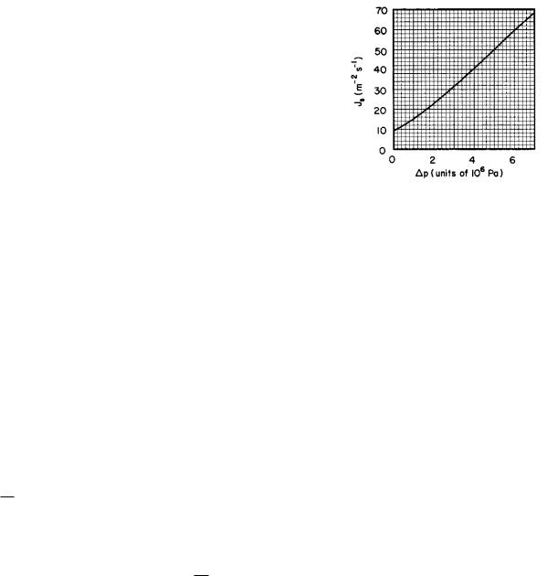
Problem 23 (a) Write Js in terms of Cs, Cs, Jv and x.

(b) Specialize to the case Cs = 0.

Problem 24 (a) Find the ratio (1 −σ)CsJv /[ωRT (Cs −

Cs)] in terms of x, Cs, and Cs.

(b) Specialize to the case Cs = 0 and discuss limiting values for small and large x.

Problem 25 (a) Show that

where x = Jv (1 − σ)/ωRT .

(b)Discuss the special case Cs = 0 in the limits x → 0 and x→ ∞.

(c)From the data shown, estimate Lp and ωRT . The data are for the transport of radioactive water with a concentration of 1015 molecules m−3 on one side of the membrane and zero on the other.

Problem 26 Consider the following cases for transport of water through a membrane.

(a) Water flows by bulk flow through the membrane with ∆p = 0. There is an impermeant solute (σ = 1) on the right with concentration Cbig and zero concentration on the left. Find the particle fluence rate of water in terms of Lp.

(b)There is no volume flow through the membrane (Jv = 0). Some of the water molecules on the left are tagged with radioactive hydrogen (tritium). The concentration of tagged water molecules is Cs on the left and 0 on the right. Find the particle fluence rate of tagged water in terms of Lp and ωRT .

(c)There is volume flow, as in case (a), and there are also tagged water molecules on the left. Find the particle fluence rate of tagged water in terms of Lp and ωRT .

(d)Restate the answers in terms of the parameters of a collection of n pores per unit area of radius Rp and length

∆Z.

(e)Estimate the value of x for part (c) if Rp = 10−8 m and cbig = cs =0.1 mol 1−1.

Problem 27 Construct diagrams analogous to Fig. 5.17

(a) when the total pressure is the same on both sides and π = 0 and (b) when (p − σπ) < p and π = 0.

Problem 28 Consider the case of water permeability shown in Fig. 5.1(c). Water and solute molecules move through the membrane in the same way. They “dissolve” from solution into the membrane. Assume that the concentration of water molecules just inside the membrane is proportional to the pressure just outside: C = αp. The membrane has thickness ∆Z and the di usion constant for water in the membrane material is D. Under steadystate conditions, derive an expression for Lp.

Problem 29 Consider the case in which solute moves along a tube by a combination of di usion and solvent drag. Ignore radial di usion within the tube, but assume that solute is moving out through the walls so that js is changing with position in the tube. In particular, the number of solute particles passing out through the wall in length dz in time dt is CA2πRp dz dt, where A is related to the permeability of the wall. Consider a case in

which C does not change with time, but depends only on position along the tube.

(a) Write down the conservation equation for an element of the tube and show that

−∂j − 2AC = 0. ∂z Rp

(b) Combine the results of part (a) with Eq. 5.45a and show that C(z) must satisfy the di erential equation

∂2C − jv f ∂C − 2A C = 0. ∂z2 D ∂z DRp

Show that this equation will be satisfied if the concentration decreases exponentially along the tube as C(z) = C0e−αz , where

Problem 30 The volume of a water molecule is Vw and the volume of a solute molecule is Vs. Define a new quantity Jw that is the number of water molecules per unit area per second passing through the membrane. What is Jw in terms of Jv and Js?

References

Basser, P. J., R. Schneidermann, R. A. Bank, E. Wachtel, and A. Maroudas (1998). Mechanical properties of the collagen network in human articular cartilage as measured by osmotic stress technique. Arch. Biochem. Biophys. 351: 207–219.

Bean, C. P. (1969). Characterization of Cellulose Acetate Membranes and Ultrathin Films for Reverse Osmosis. Research and Development Progress Report No. 465 to the U.S. Department of Interior, O ce of Saline Water. Contract No. 14-01-001-1480. Washington, Superintendent of Documents, October 1969.

Bean, C. P. (1972). The physics of porous membranes: Neutral pores, in G. Essenman, ed., Membranes. New York, Dekker, Vol. 1, pp. 1–55.

Beck, R. E., and J. S. Schultz (1970). Hindered di u- sion in microporous membranes with known pore geometry. Science 170: 1302–1305.

Calland, C. H. (1972). Iatrogenic problems in end-stage renal failure. N. Engl. J. Med. 287: 334–336.

Cokelet, G. R. (1972). The rheology of human blood, in Y. C. Fung et al., eds. Biomechanics: Its Founda-

References 133

tions and Objectives. Englewood Cli s, NJ, Prentice Hall (especially p. 77, Fig. 4).

Durbin, R. P. (1960). Osmotic flow of water across permeable cellulose membranes. J. Gen. Physiol. 44: 315– 326.

Fishman, R. A. (1975). Brain edema. N. Engl. J. Med. 293: 706–711.

Galletti, P. M., C. K. Colton, and M. J. Lysaght (2000). Artificial kidney. In J. D. Bronzino, ed. The Biomedical Engineering Handbook, 2nd. ed., Vol. 2. Boca Raton, FL CRC Press.

Gennari, F. J., and J. P. Kassirer (1974). Osmotic diuresis. N. Engl. J. Med. 291: 714–720.

Guyton, A. C. (1991). Textbook of Medical Physiology,

8th ed. Philadelphia, Saunders.

Guyton, A. C., A. E. Taylor, and H. J. Granger (1975).

Circulatory Physiology II. Dynamics and Control of the Body Fluids. Philadelphia, Saunders.

Hildebrand, J. H., and R. L. Scott (1964). The Solubility of Nonelectrolytes. 3rd ed. New York, Dover.

Katchalsky, A., and P. F. Curran (1965). Nonequilibrium Thermodynamics in Biophysics. Cambridge, Harvard University Press.

Levitt, D. G. (1975). General continuum analysis of transport through pores. I. Proof of Onsager’s reciprocity postulate for uniform pore. Biophys. J. 15: 533– 551.

Lindner, A., B. Charra, D. J. Sherrard, and B. H. Scribner (1974). Accelerated atherosclerosis in prolonged maintenance hemodialysis. N. Engl. J. Med. 290: 697– 701.

Lysaght, M. J., and J. Moran (2000). Peritoneal dialysis equipment. In J. D. Bronzino, ed. The Biomedical Engineering Handbook. 2nd ed., Vol. 2. Boca Raton, FL, CRC Press.

Patton, H. D., A. F. Fuchs, B. Hille, A. M. Scher, and R. F. Steiner, eds. (1989). Textbook of Physiology, 21st ed. Philadelphia, Saunders.

Schmidt-Nielsen, K. (1972). How Animals Work. Cambridge, Cambridge University Press.

Silverstein, M. E., C. A. Ford, M. J. Lysaght, and L. W. Henderson (1974). Treatment of severe fluid overload by ultrafiltration. N. Engl. J. Med. 291: 747–751.

Steinmuller, D. R. (1998). A dangerous error in the dilution of 15 percent albumin. N. Engl. J. Med. 338: 1226.

Thomas, Lewis (1974). Lives of a Cell. New York, Viking.

White, R. J., and M. J. Likavek (1992). Current concepts: The diagnosis and initial management of head injury. N. Engl. J. Med. 327: 1502–1511.

A nerve cell conducts an electrochemical impulse because of changes that take place in the cell membrane. These changes allow movement of ions through the membrane, setting up currents that flow through the membrane and along the cell. Similar impulses travel along muscle cells before they contract. This chapter reviews the basic properties of electric fields and currents that are needed to understand the propagation of the nerveor muscle-cell impulse.

Section 6.1 introduces the physiology of nerve conduction. The next eight sections develop the electrostatics and the physics of current flow needed to understand how the action potential propagates along the cell.

The next sections deal with the charge distribution on a resting cell membrane (Sec. 6.10) and the cable model of the axon (Sec. 6.11). If the membrane properties do not change as the voltage across the membrane changes, this leads to electrotonus or passive spread (Sec. 6.12). If the membrane properties do change, a signal can propagate without change of shape. Section 6.13 tells how Hodgkin and Huxley developed equations to describe the membrane changes, and Secs. 6.14 and 6.15 apply their results to the propagation of a nerve impulse. The chapter to this point forms an integrated story of conduction in an unmyelinated axon.

Section 6.16 considers saltatory conduction: the “jumping” of an impulse from node to node in a myelinated fiber. Section 6.17 examines the capacitance of a bilayer membrane that has layers with di erent properties. Section 6.18 shows how minor alterations in the membrane properties can transform the Hodgkin–Huxley model to one that displays repetitive electrical activity.

Section 6.19 shows how tabulated solutions to the electrical capacitance of conductors in di erent geometries can be used to solve di usion problems with similar geometric configurations.

6.1Physiology of Nerve and Muscle Cells

A nerve1 consists of many parallel, independent signal paths, each of which is a nerve cell or fiber. Each cell transmits signals in only one direction; separate cells carry signals to or from the brain. Each cell has an input end (dendrites), a cell body, a long conducting portion or axon, and an output end. It is the ends that give the cell its unidirectional character. The input end may be a transducer (stretch receptor, temperature receptor, etc.) or a junction (synapse) with another cell. A threshold mechanism is built into the input end; when an input signal exceeding a certain level is received, the nerve fires and an impulse or action potential of fixed size and duration travels down the axon. There may be several inputs that can either aid or inhibit each other, depending on the nature of the synapses.

Muscle cells are also long and cylindrical. An electrical impulse travels along a muscle cell to initiate its contraction. This chapter concentrates on the propagation of the action potential in a nerve cell, but the discussion can be regarded as a model for what happens in muscle cells as well.

The axon transmits the impulse without change of shape. The axon can be more than a meter in length, extending from the brain to a synapse low in the spinal cord or from the spinal cord to a finger or toe. Bundles of axons constitute a nerve. The output end branches out in fine nerve endings, which appear to be separated by a gap from the next nerve or muscle cell that they drive.

1A good discussion of the properties of nerves and the Hodgkin– Huxley experiments is found in Katz (1966). More modern descriptions of nerves and nerve conduction are found in many books, such as Patton et al. (1989).

136 6. Impulses in Nerve and Muscle Cells

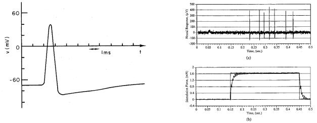
FIGURE 6.1. A typical nerve impulse or action potential, plotted as a function of time.

The long cylindrical axon has properties that are in some ways similar to those of an electric cable. Its diameter may range from less than one micrometer (1 µm) to as much as 1 mm for the giant axon of a squid; in humans the upper limit is about 20 µm. Pulses travel along it with speeds ranging from 0.6 to 100 m s−1, depending, among other things, on the diameter of the axon. The axon core may be surrounded by either a membrane (for an unmyelinated fiber) or a much thicker sheath of fatty material (myelin) that is wound on like tape. A myelinated fiber has its sheath interrupted at intervals and replaced by a short segment of membrane similar to that on an unmyelinated fiber. These interruptions are called nodes of Ranvier . A typical human nerve might contain twice as many unmyelinated fibers as myelinated. We will see in Sec. 6.16 that the myelin gives a faster impulse conduction speed for a given axon radius. Myelinated fibers conduct motor information; unmyelinated fibers conduct information such as temperature, for which speed is not important. A typical unmyelinated axon might have a radius of 0.7 µm with a membrane thickness of 5–10 nm. Myelinated fibers have a radius of up to 10 µm, with nodes spaced every 1–2 mm. We will find later that the spacing of the nodes is about 140 times the inner radius of the fiber, a fact that is quite important in the relationship between conduction speed and fiber radius.

A microelectrode inserted inside a resting axon shows an electrical potential that is about 70 mV less than outside the cell. (We will define electrical potential di erence in Sec. 6.4.) A typical nerve impulse or action potential or spike in an unmyelinated axon is shown as a function of time in Fig. 6.1. As the impulse passes by the electrode, the potential rises in a millisecond or less to about +40 mV. The potential then falls to about −90 mV and then recovers slowly to its resting value of −70 mV. The membrane is said to depolarize and then repolarize.

The history of recording the action potential has been described by Geddes (2000). The action potential was first measured by Helmholtz around 1850. The measure-

FIGURE 6.2. The response of a mechanical receptor in the cornea to an applied force. (a) The impulses recorded on the surface of the nerve bundle. (b) The applied force. Impulses occur while the force is applied. From B. J. Kane, C. W. Storment, S. W. Crowder, D. L. Tanelian, and G. T. A. Kovacs. Force-sensing microprobe for precise stimulation of mechanoreceptive tissues. IEEE Trans. Biomed. Eng. 42(8):745–750. c 1995 IEEE. Reprinted by permission.

ment technology steadily improved, culminating in the use of a microelectrode inserted by Hodgkin and Huxley (1939) into the cut end of the giant axon of the squid, to record the action potential directly.

The information sent along a nerve fiber is coded in the repetition rate of these pulses, all of which are the same shape. Figure 6.2 shows the response of a low-threshold mechanoreceptor in the cornea to a mechanical stimulus. The heavy curve in the bottom panel shows the applied force, and the upper panel shows the impulses.

Comparison of the intracellular fluid or axoplasm with the extracellular fluid surrounding each axon shows an excess of potassium and a deficit of sodium and chloride ions within the cell, as shown in Fig. 6.3. The regenerative action that produces the sudden changes of membrane potential is caused by changing permeability of the membrane to ions—primarily sodium and potassium. These changes are discussed in Secs. 6.13 and 6.14.

The axon can be removed from the rest of the cell and it will still conduct nerve impulses. The speed and shape of the action potential depend on the membrane and the concentration of ions inside and outside the cell. The axoplasm has been squeezed out of squid giant axons and replaced by an electrolyte solution without altering appreciably the propagation of the impulses—for a while, until the ion concentrations change appreciably. The axoplasm does contain chemicals essential to the long-term metabolic requirements of the cell and to maintaining the ion concentrations.

At the end of a nerve cell the signal passes to another nerve cell or to a muscle cell across a synapse or junction. A few synapses in mammals are electrical; most are