

Intermediate Physics for Medicine and Biology - Russell K. Hobbie & Bradley J. Roth
.pdf11.6 The Power Spectrum |
297 |
n = 3; Q = 0.102 |
(a) |
Gibbs phenomenon |
n = 39; Q = 0.013 |
(b) |
FIGURE 11.16. Fit to the square wave. (a) Fit with the terms for k = 1 and k = 3. The value of Q is 0.102. (b) Fit with terms through k = 39. Q is very small, but the Gibbs phe- nomenon—spikes near the discontinuity—is apparent.
power. A periodic signal y(t) can be written as
n
y(t) = a0 + [ak cos(kω0t) + bk sin(kω0t)] + n(t),
k=1
(11.35) where the error n(t) is the di erence between the signal (represented by an infinite number of terms) and the sum over n terms. [This equation defines n(t). n(t) does not represent “noise,” which is discussed in a later section.] The coe cients are given by Eqs. 11.33.
The average “power” in the signal is defined to be3
3y24 |
= lim |
1 |
T |
y2(t) dt. |
(11.36) |
|
|||||
|
T →∞ 2T |
−T |
|
|
|
For a periodic signal, the same result can be obtained by integrating over one period:
3y24 |
= |
1 |
T y2(t) dt. |
(11.37) |
|
||||
|
|
T 0 |
|
|
To calculate this using Eq. 11.35 for y(t), we have to write the sum twice and multiply both sums together:
1 |
T y2(t) dt = |
1 |
T |
||
|
|
||||
T 0 |
|
|
T 0 |
||
|
|
n |
|
! |
|
|
a0 |
+ [ak cos(kω0t) + bk sin(kω0t)] + n(t) |
|||
|
|
k=1 |
|
|
|
|
|
n |
|
|
|
|
|
|
[aj cos(jω0t) + bj sin(jω0t)] + n(t) dt. |
||
× a0 + |
|||||
j=1
3The time average of a variable will be denoted by brackets.
FIGURE 11.17. Analysis of the pulmonary arterial blood flow in a dog, in terms of a Fourier series. From W. R. Milnor, Pulsatile blood flow. New Eng. J. Med. 287: 27–34. Copyrightc Massachusetts Medical Society. All rights reserved. Drawing courtesy of Professor Milnor.
When these terms are multiplied together and written out, we have
y |
2 |
= |
|
1 |
T |
|
|
|
|
|
T |
0 |
|
|
|
|
|||
|
|
(i) |
|
|
|
n |
(ii) |
(iii) |
|
dt |
|
a02 |
+ 2a0 |
ak cos(kω0t) + bk sin(kω0t) |
|
||||
|
|
|
|
|
|
k=1 |
|
|
|
|
|
(iv) |
|
n |
(v) |
(vi) |
|
||
+ 2a0 n(t) + a2k cos2(kω0t) + b2k sin2(kω0t)
|
k=1 |
n |
(vii) |
|
+ak aj cos(kω0t) cos(jω0t)
k=1 j =k |
|
n |
(viii) |
+bk bj sin(kω0t) sin(jω0t)
k=1 j |
=k |
|
|
n |
n |
(ix) |
|
|
|
|
|
+ 2 akbj cos(kω0t) sin(jω0t) |
|
||
k=1 j=1 |
|
|
|
|
n |
(x) |
(xi) ! |
|
|
||
+ 2 n(t) ak cos(kω0t) + bk sin(kω0t) |
+ n2 (t) . |
||
k=1
298 |
11. The Method of Least Squares and Signal Analysis |
||||||||||||||
|
1.0 |
|
|
|
|
|
|
|
|
|
|
|
|
|
|
|
|
|
|
|
|
|
|
|
|
|
|
|
|
|
|
)/2 |
0.8 |
|
|
|
|
|
|
|
|
|
|
|
|
|
|
|
|
|
|
|
|
|
|
|
|
|
|
|
|
||
|
|
|
|
|
|
|
|
|
|
|
|
|
|
|
|
2 k |
0.6 |
|
|
|
|
|
|
|
|
|
|
|
|
|
|
+b |
|
|
|
|
|
|
|
|
|
|
|
|
|
|
|
|
|
|
|
|
|
|
|
|
|
|
|
|
|
||
|
|
|
|
|
|
|
|
|
|
|
|
|
|
|
|
2 k |
|
|
|
|
|
|
|
|
|
|
|
|
|
|
|
(a |
0.4 |
|
|
|
|
|
|
|
|
|
|
|
|
|
|
|
|
|
|
|
|
|
|
|
|
|
|
|
|
||
= |
|
|
|
|
|
|
|
|
|
|
|
|
|
|
|
k |
|
|
|
|
|
|
|
|
|
|
|
|
|
|
|
Φ |
0.2 |
|
|
|
|
|
|
|
|
|
|
|
|
|
|
|
|
|
|
|
|
|
|
|
|
|
|
|
|
||
|
0.0 |
|
|
|
|
|
|
|
|
|
|
|
|
|
|
|
|
|
|
|
|
|
|
|
|
|
|
|
|
|
|
|
|
|
|
|
|
|
|
|
|
|
|
|
|
|
|
|
1 |
3 |
5 |
7 |
9 |
|
|
|
|||||||
k
FIGURE 11.18. The power spectrum Φk for the square wave of Fig. 11.6 or Fig. 11.17, calculated using the values of bk from Table 11.4.
Each term has been labeled (i) through (xi). Assume that the function y is su ciently well behaved so that the order of integration and summation can be interchanged. Term (i) gives a20. Terms (ii) and (iii) are integrals of the cosine or sine over an integral number of cycles and vanish. Term (iv) gives4
2a0 |
1 |
T n(t) dt = 0. |
|
||
|
T 0 |
|
y1(t) y2(t)
|
|
|
|
|
(a) |
|
|
|
|
|
|
|
|
|
y2(t + τ) |
|
|
|
|
|
|
|
|
|
|
|
|||
|
|
|
|
|
|
τ = 1 |
|
|
|
|
||||
y1(t)y2(t + τ) |
|
|
|
|
|
|
|
|
|
|
|
|
|
|
|
|
|
|
|
|
|
|
|
|
|
|
|||
y2(t + τ) |
|
|
|
|
|
|
|
|
|
|
|
|
|
|
|
|
|
|
|
τ = 1.5 |
|
|
|
|
|
||||
y1(t)y2(t + τ) |
|
|
|
|
|
|
|
|
|
|
|
|
|
|
|
|
|
|
|
|
|
|
|
|
|
|
|
|
|
|
|
|
|
|
|
|
|
|
|
|
|
|
|
|
y2(t + τ) |
|
|
|
τ = 2.0 |
|
|
|
|
||||||
|
|
|
|
|
|
|
|
|
|
|
|
|
||
y1(t)y2(t + τ) |
|
|
|
|
|
|
|
|
|
|
|
|
|
|
|
|
|
|
|
|
|
|
|
|
|
|
|
|
|
|
|
|
|
|
|
|
|
|
|
|
|
|
|
|
y2(t + τ) |
|
|
|
τ = 2.5 |
|
|
|
|
|
|
|
|
||
|
|
|
|
|
|
|
|
|
|
|
|
|
||
y1(t)y2(t + τ |
) |
|
|
|
|
|
|
|
|
|
|
|
|
|
|
|
|
|
|
|
|
|
|
|
|
|
|
|
|
0 |
2 |
4 |
|
t |
6 |
8 |
||||||||
|
|
|
|
|
(b) |
|
|
|
|
|
|
|||
|
|
|
|
|
|
|
|
|
|
|
|
|
||
Terms (v) and (vi) give a2k /2 and b2k/2. Terms (vii), (viii), and (ix) all vanish because of Eq. 11.32. Terms like (x) vanish because n(t) can be approximated by a sum of sine and cosine terms extending from k = n+1 to infinity that are orthogonal to terms for 1 < k < n. Term (xi) is 3 2n4. We finally have for the average power
|
|
|
|
1 |
n |
|
|
|
|
n |
|
|
2 |
|
2 |
|
|
2 |
2 |
2 |
4 = |
|
2 |
|
|
3y |
(t)4 |
= a0 |
+ |
2 |
k=1 |
(ak |
+ bk ) + |
3 n |
k=0 |
Φk + 3 n |
4 . |
|
|
|
|
|
|
|
|
|
|
|
|
(11.38) The coe cients are defined by Eqs. 11.33. We could have made a similar argument for the discrete Fourier series of Eqs. 11.25 or 11.26 and obtained the same result. In both cases the average power is a sum of terms Φk that represent the average power at each frequency kω0. The term Φ0 = a20 is the average of the square of the zerofrequency or dc (direct-current) term; Φk = (a2k + b2k )/2 is the average of the squares of the terms ak cos(kω0t) and bk sin(kω0t); and 3 2n4 is the average of the square of the error term. Figure 11.18 shows the power spectrum of the square wave that was used in the example.
11.7 Correlation Functions
The correlation function is useful to test whether two functions of time are correlated, that is, whether a change
4The quantity y(t) −a0 has an average of zero. Since all the sine and cosine terms have an average of zero, n also has an average of zero.
φ12(τ)
-4 |
-2 |
0 |
2 |
τ 4 |
|
|
(c) |
|
|
FIGURE 11.19. An example of the cross-correlation function.
(a) The two signals to be correlated. (b) Plots of y2(t + τ ) and the product y1(t)y2(t + τ ) for di erent values of τ . (c) Plot of φ12(τ ). The peak occurs when signal y2 has been advanced 2 s.
in one is accompanied by a change in the other. Let the two variables to be tested be y1(t) and y2(t). The change in y2 may occur earlier or later than the change in y1; therefore the correlation must be examined as one of the variables is shifted in time. Examples of pairs of variables that may be correlated are wheat price and rainfall, urinary output and fluid intake, and the voltage changes at two di erent points along the nerve axon. The variables may or may not be periodic. Exhibiting a correlation does not establish a cause-and-e ect relationship. (The height of a growing tree may correlate for several years with an increase in the stock market.)
11.7.1Cross-Correlation of a Pulse
To calculate the cross-correlation function of y1 and y2, advance y2(t) by an amount τ , multiply y1 by the shifted y2, and integrate the product. Figure 11.19 shows the process for two pulses. The second pulse occurs 2 s later than the first. As the second pulse is advanced the pulses
begin to overlap. When the second pulse has been advanced by 2 s the overlap is greatest; as it is advanced more, the overlap falls to zero. The cross-correlation function depends on τ and is plotted in Fig. 11.19(c). The mathematical statement of this procedure for a pulse is
|
∞ |
|
φ12(τ ) = |
y1(t)y2(t + τ ) dt. |
(11.39) |
|
−∞ |
|
The integrand makes a positive contribution to the integral if y1(t) and y2(t + τ ) are both positive at the same time or both negative at the same time. It makes a negative contribution if one function is positive while the other is negative.
11.7 Correlation Functions |
299 |
y1(t)
y2(t+τ)
y1(t)y2(t+τ)
(a) τ = 0; φ12 > 0
y1(t)
y2(t+τ)
11.7.2 Cross-Correlation of a Nonpulse Signal
If the signals are not pulses, then the cross-correlation integral is defined as
φ12(τ ) = y1(t)y2(t + τ ) . |
(11.40) |
As before, the average is the integral over a long time divided by the time interval:
1 |
T |
|
|
φ12(τ ) = lim |
|
y1(t)y2(t + τ ) dt. |
(11.41) |
|
|||
T →∞ 2T |
−T |
|
|
If the signals have period T , the average can be taken by integrating over a single period:
φ12(τ ) = |
1 |
t +T y1(t)y2(t + τ ) dt. |
(11.42) |
|
T |
||||
|
t |
|
||
|
|
|
Note the di erence in units between φ12 as defined for pulses in Eq. 11.39 where the units of φ are the units of y2 times time, and φ12 defined in Eqs. 11.40–11.42 where the units are those of y2.
The cross correlation depends only on the relative shift of the two signals. It does not matter whether y2 is advanced by an amount τ or y1 is delayed by the same amount:
φ21(−τ ) = φ12(τ ). |
(11.43) |
11.7.3 Cross-Correlation Example
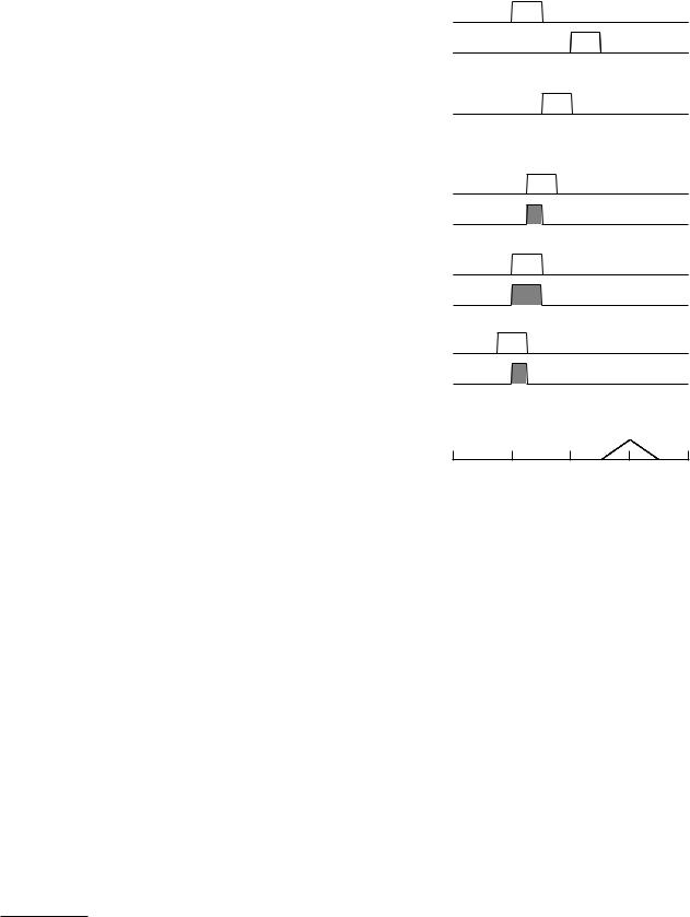
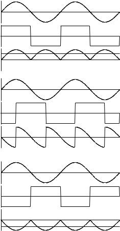
As an example of the cross correlation, consider a square wave that has value ±1 and a sine wave with the same period (Fig. 11.20). When the square wave and sine wave are in phase, the product is always positive and the cross correlation has its maximum value. As the square wave is shifted the product is sometimes positive and sometimes negative. When they are a quarter-period out of phase, the average of the integrand is zero, as shown in Fig. 11.20(b). Still more shift results in the correlation function becoming negative, then positive again, with a shift of one full period giving the same result as no shift.
y1(t)y2(t+τ)
(b) τ = 3T/4 or -T/4; φ12 = 0
y1(t)
y2(t+τ)
y1(t)y2(t+τ) |
|
|
(c) |
τ = ± T/2; |
φ12 < 0 |
FIGURE 11.20. Cross correlation of a square wave and a sine wave of the same period.
11.7.4 Autocorrelation
The autocorrelation function is the correlation of the signal with itself:
|
|
|
φ11(τ ) = y1(t)y1(t + τ ) dt |
(pulse), |
(11.44) |
φ11(τ ) = y1(t)y1(t + τ ) |
(nonpulse). |
(11.45) |
Since the signal is correlated with itself, advancing one copy of the signal is the same as delaying the other. The autocorrelation is an even function of τ :
φ11(τ ) = φ11(−τ ). |
(11.46) |
11.7.5 Autocorrelation Examples
The autocorrelation function for a sine wave can be calculated analytically. If the amplitude of the sine wave is
300 11. The Method of Least Squares and Signal Analysis
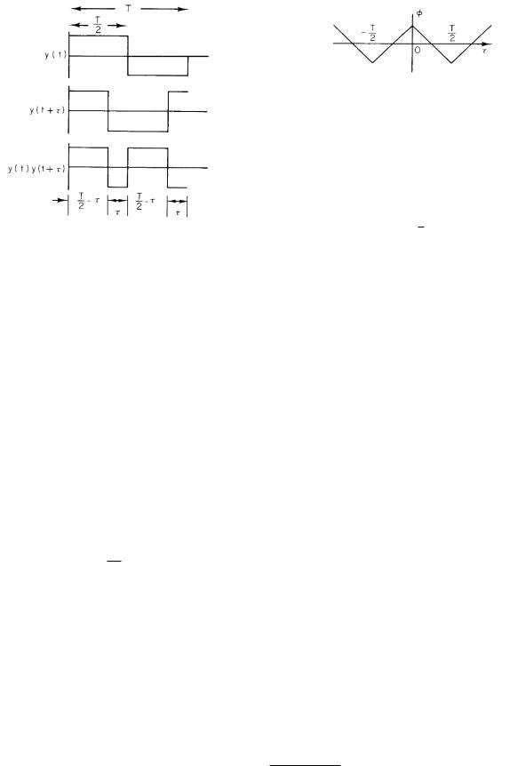
FIGURE 11.22. Plot of φ11(τ ) for the square wave.
FIGURE 11.21. Plots of y(t), y(t + τ ), and their product for a square wave.
A and the frequency is ω = 2π/T ,
φ11(τ ) = |
A2 |
T sin(ωt) sin(ωt + ωτ ) dt |
|
T |
|||
|
0 |
||
= |
A2 |
T sin(ωt) |
|
T |
|||
|
0 |
× [sin(ωt) cos(ωτ ) + cos(ωt) sin(ωτ )] dt
11.8The Autocorrelation Function and the Power Spectrum
We saw that the power spectrum of a periodic signal is related to the coe cients in its Fourier series (Eq. 11.38):
n
3y2(t)4 = a20 + 12 (a2k + b2k),
k=1
with the term for each value of k representing the amount of power carried in the signal component at that frequency. The Fourier series for the autocorrelation function carries the same information. To see this, calculate the autocorrelation function of
n
y1(t) = a0 + [ak cos(kω0t) + bk sin(kω0t)] .
k=1
We can write
|
= A |
2 |
|
1 |
|
T |
|
2 |
|
φ11(τ ) = y1(t)y1(t + τ ) |
|
|||||
|
|
cos(ωτ ) |
|
|
|
|
|
|
sin |
|
(ωt) dt |
5 |
n |
|
! |
|
|
|
|
T |
|
|
|
|
|
||||||||
|
|
|
|
|
0 |
|
|
|
|
= |
a0 + [ak cos(kω0t) + bk sin(kω0t)] |
|||||
|
+ A2 sin(ωτ ) |
|
|
1 |
|
T |
|
|
|
|
k=1 |
|
|
|||
|
|
|
sin(ωt) cos(ωt) dt . |
|
n |
% |
|
|||||||||
|
|
|
|
|
||||||||||||
|
|
|
|
|
T |
0 |
|
|
|
|
|
|
aj cos[jω0(t + τ )] |
|||
|
|
|
|
|
|
|
|
|
|
|
|
|
× a0 + |
|||
It is shown |
1in Appendix E that the first term in square |
|
j=1 |
|
|
|||||||||||
|
|
|
6!7 |
|||||||||||||
brackets is |
2 and the second is 0. Therefore the autocor- |
+ bj sin[jω0(t + τ )] |
. |
|||||||||||||
relation function of the sine wave is |
|
|
|
|
|
|||||||||||
|
A2 |
|
φ11(τ ) = |
2 cos(ωτ ). |
(11.47) |
As a final example, consider the autocorrelation of a square wave of unit amplitude. One period is drawn in Fig. 11.21 showing the wave, the advanced wave, and the product. The average is the net area divided by T . The area above the axis is (2)(T /2 −τ )(1) since there are two rectangles of height 1 and width T /2 −τ . From this must be subtracted the area of the two rectangles of height 1 and width τ that are below the axis. The net area is T − 4τ . The autocorrelation function is
φ11(τ ) = 1 − 4τ /T, 0 < τ < T /2. |
(11.48) |
The plot of the integrand in Fig. 11.21 is only valid for 0 < τ < T /2. We can use the fact that the autocorrelation is an even function to draw φ for −T /2 < τ < 0. We then have φ for the whole period. It is plotted in Fig. 11.22.
The next step is to multiply out all the terms as we did when deriving Eq. 11.38. We then use the trigonometric identities5
cos(x + y) = cos x cos y − sin x sin y,
sin(x + y) = cos x sin y + sin x cos y.
For many of the terms, either the averages are zero or pairs of terms cancel. We finally obtain
|
n |
|
|
|
|
φ11(τ ) = a02 + |
|
1 |
(ak2 |
+ bk2 ) cos(kω0τ ). |
(11.49) |
|
|||||
|
2 |
|
|
|
|
k=1
This has only cosine terms, since the autocorrelation function is even.
5One virtue of the complex notation is that these addition formulae become the standard rule for multiplying exponentials: ei(x+y) = eixeiy .
11.9 Nonperiodic Signals and Fourier Integrals |
301 |
Fourier series
y (t) |
|
|
|
ak ,bk |
|
||
|
|
|
|||||
|
|
|
|
|
|||
Auto- |
|
|
|
Φk = 21 (ak2 |
+ bk2 ) |
||
correlation |
|
|
|
||||
|
|
|
Fourier series |
|
|
Power |
|
φ11(τ ) |
|
|
|
||||
|
|
Φk spectrum |
|
||||
|
|
|
|||||
(discrete)
FIGURE 11.23. The power spectrum of a periodic signal can be obtained either from the squares of the Fourier coe cients of the signal or from the Fourier coe cients of the autocorrelation function.
For zero shift,
n
φ11(0) = a20 + 12 (a2k + b2k ).
k=1
Comparison with Eq. 11.38 shows that this is the power in the signal. We can get this result directly from Eq. 11.36. The integral is the same as the definition of the autocorrelation function when τ = 0.
The Fourier series for the autocorrelation function is particularly easy to obtain. We need only pick out the coe cients in Eq. 11.49. Write the Fourier expansion of the autocorrelation function as
n |
|
φ11(τ ) = α0 + αk cos(kω0τ ). |
(11.50) |
k=1
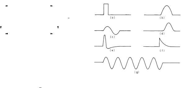
FIGURE 11.24. Various pulses. The common feature is that they occur once. (a) Square pulse. (b) Half cycle of a sine wave. (c) One cycle of a sine wave. (d) Gaussian. (e) Nerve pulse. (f) Exponentially decaying pulse. (g) Gated sine wave.
11.9Nonperiodic Signals and Fourier Integrals
Sometimes we have to deal with a signal that is a pulse that occurs just once. Several pulses are shown in Fig. 11.24; they come in an infinite variety of shapes. Noise is another signal that never repeats itself and is therefore not periodic. The Fourier integral or Fourier transform is an extension of the Fourier series that allows us to deal with nonperiodic signals.
Comparing terms in Eqs. 11.49 and 11.50 shows that α0 = a20 and αk = (a2k + b2k )/2. We can also compare these with the definition of Φk in Eq. 11.38 and say that
Φ0 = average dc (zero- |
= α0 = a02, |
|
|
frequency) power |
|
|
|
Φk = average power at |
= αk = 1 |
(a2 |
+ b2 ). |
|
2 |
k |
k |
frequency kω0
(11.51) The autocorrelation function contains no phase information about the signal. This is reflected in the fact that αk = (a2k + b2k ); the sine and cosine terms at a given frequency are completely mixed together.
There are two ways to find the power Φk at frequency kω0. Both are shown in Fig. 11.23. The function y(t) and its Fourier coe cients are completely equivalent, and one can go from one to the other. Squaring the coe cients and adding them gives the power spectrum. This is a one-way process; once they have been squared and added, there is no way to separate them again. The autocorrelation function also involves squaring and adding and is a oneway process. The autocorrelation function and the power spectrum are related by a Fourier series and can be calculated from each other.
11.9.1Introduce Negative Frequencies and Make the Coe cients Half as Large
The Fourier series expansion of a periodic function y(t) was seen in Eq. 11.30. If we let the number of terms be infinite, we have
∞ |
∞ |
y(t) = a0 + ak cos(kω0t) + |
bk sin(kω0t), |
k=1 |
k=1 |
with the coe cients given by Eqs. 11.33. Since y(t) has period T , the integrals in Eqs. 11.33 can be over any interval that is one period long. Let us therefore make the limits of integration −T /2 to T /2 and also remember that 1/T = ω0/2π. With these substitutions, Eqs. 11.33 become
|
|
a0 = |
|
ω0 |
T /2 |
y(t) dt, |
|
|||
|
|
|
2π |
|
||||||
|
|
|
|
|
|
−T /2 |
|
|
||
|
|
|
|
|
|
|
|
|
||
ak = |
ω0 |
T /2 y(t) cos(kω0t) dt, |
(11.52) |
|||||||
π |
||||||||||
|
|
−T /2 |
|
|
|
|||||
bk = |
ω0 |
T /2 y(t) sin(kω0t) dt. |
|
|||||||
π |
|
|||||||||
|
|
|
|
−T /2 |
|
|
||||
302 11. The Method of Least Squares and Signal Analysis
Now allow k to have negative as well as positive values. If the coe cients for negative k are also defined by Eqs. 11.52, they have the properties [since cos(kω0t) = cos(−kω0t) and sin(kω0t) = − sin(−kω0t)],
a−k = ak, b−k = −bk .
Therefore the terms ak cos(kω0t) and bk sin(kω0t) in Eq. 11.30 are the same function of t whether k is positive or negative. By introducing negative values of k we can make the coe cients in front of the integrals for ak and bk in Eqs. 11.52 become ω0/2π. This is the same trick used to obtain the discrete equations, Eqs. 11.27. With negative values of k allowed, we have
∞
y(t) = a0 + [ak cos(kω0t) + bk sin(kω0t)] ,
k=−∞ k =0
FIGURE 11.25. (a) A periodic signal. (b) A nonperiodic signal.
a0 = ω0 T /2 y(t) dt,
2π −T /2
ak = ω0 T /2 y(t) cos(kω0t) dt,
2π −T /2
bk = ω0 T /2 y(t) sin(kω0t) dt.
2π −T /2
Since cos(0ω0t) = 1 and sin(0ω0t) = 0, we can incorporate the definition of a0 into the definition of ak and introduce b0 which is always zero. The sum can then include k = 0:
∞
y(t) = [ak cos(kω0t) + bk sin(kω0t)] ,
k=−∞
a |
= |
ω0 |
|
T /2 |
y(t) cos(kω |
0 |
t) dt, |
(11.53) |
|||||
|
|||||||||||||
k |
2π |
|
−T /2 |
|
|
|
|
|
|
||||
|
|
|
|
|
|
|
|
|
|||||
|
b = |
|
ω0 |
T /2 |
y(t) sin(kω |
0 |
t) dt. |
|
|||||
|
2π |
|
|||||||||||
|
k |
−T /2 |
|
|
|
|
|
||||||
|
|
|
|
|
|
|
|
|
|
||||
A final change of variables defines Ck = 2πak /ω0 and Sk = 2πbk /ω0. With these changes the Fourier series and its coe cients are
|
ω0 |
∞ |
|
|
y(t) = |
|
[Ck cos(kω0t) + Sk sin(kω0t)] , |
||
|
||||
|
2π |
|
||
|
|
k=−∞ |
|
|
|
|
T /2 |
|
|
FIGURE 11.26. An approximation to the nonperiodic signal shown in Fig. 11.25(b).
11.9.2Make the Period Infinite
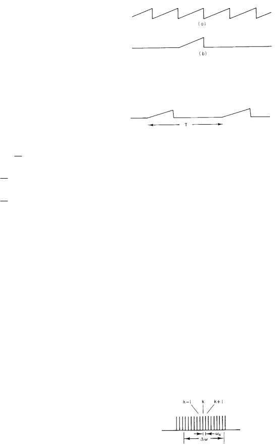
These equations can be used to calculate the Fourier series for a periodic signal such as that shown in Fig. 11.25(a). Suppose that instead we want to find the coefficients for the nonperiodic signal shown in Fig. 11.25(b). This signal can be approximated by another periodic signal shown in Fig. 11.26. The approximation to Fig. 11.25(b) becomes better and better as T is made longer. As T becomes infinite, the fundamental angular frequency ω0 approaches 0. Define ω = kω0. The frequencies ω are discrete with spacing ω0. Consider a small frequency interval encompassing many values of k, as shown in Fig. 11.27. Since ω0 is approaching zero, there can be many values of ω and k between ω and ω + ∆ω. The frequencies will be nearly the same, so the values of Ck will be nearly the same. All of the terms in the sum in Eq. 11.54 can be replaced by an average value of Ck or Sk multiplied by the number of values of k in the interval, which is ∆ω/ω0. Finally, we set Ck=C(ω) and ∆ω = dω. The sum becomes an integral with ∆ω = dω:
y(t) = |
ω0 |
∞ |
[C(ω) cos ωt + S(ω) sin ωt] |
dω |
, |
2π |
|
||||
|
−∞ |
|
ω0 |
||
Ck = |
y(t) cos(kω0t) dt, |
(11.54) |
−T /2 |
|
|
|
T /2 |
|
Sk = |
y(t) sin(kω0t) dt. |
|
|
−T /2 |
|
To recapitulate, there is nothing fundamentally new |
|
in Eq. 11.54. Negative values of k were introduced so |
|
that the sum goes over each value of |k| twice (except for |
|
k = 0). This allowed the coe cients to be made half as |
|
large. |
FIGURE 11.27. A histogram of Ck vs k. |
11.9 Nonperiodic Signals and Fourier Integrals |
303 |
or finally, since dω = 2πdf , |
|
|
|
|
|
|
|
||
|
1 ∞ [C(ω) cos ωt + S(ω) sin ωt] dω |
|
|
1.0 |
|
|
C |
|
|
y(t) = |
|
C)/(A/a) |
|
|
|
|
|||
∞ |
2π −∞ |
|
|
0.5 |
|
|
S |
|
|
|
|
|
|
|
|
|
|||
= |
[C(f ) cos(2πf t) + S(f ) sin(2πf t)] df, |
|
or |
0.0 |
|
|
|
|
|
|
(S |
|
|
|
|
||||
−∞ |
|
∞ |
(11.55) |
|
|
|
|
|
|
|
C(ω) = |
|
-0.5 |
|
|
|
|
||
|
y(t) cos ωt dt, |
|
|
-10 |
-5 |
0 |
5 |
10 |
|
|
|
−∞ |
|
|
|||||
|
|
∞ |
|
|
|
|
ω/a |
|
|
S(ω) = y(t) sin ωt dt.
−∞
These equations constitute a Fourier integral pair or Fourier transform pair. They are completely symmetric in the variables f and t and symmetric apart from the factor 2π in the variables ω and t. One obtains C(ω) or S(ω) by multiplying the function y(t) by the appropriate trigonometric function and integrating over time. One obtains y(t) by multiplying C and S by the appropriate trigonometric function and integrating over frequency.
11.9.3 Complex Notation
Using complex notation, we define
Y (ω) = C(ω) − iS(ω) |
(11.56) |
and write
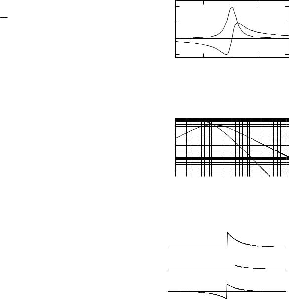
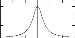
FIGURE 11.28. The sine and cosine coe cients in the Fourier transform of an exponentially decaying pulse.
|
1 |
|
|
|
|
|
|
|
|
|
|
|
|
|
4 |
|
|
|
|
|
|
|
|
|
|
|
|
C)/(A/a) |
2 |
|
|
|
|
|
|
|
S |
|
|
|
|
0.1 |
|
|
|
|
|
|
|
|
|
|
|
||
|
|
|
|
|
|
|
|
|
|
|
|
||
4 |
|
|
|
|
|
|
|
|
|
|
|
|
|
2 |
|
|
|
|
|
|
|
|
|
|
|
|
|
or |
|
|
|
|
|
|
|
C |
|
|
|
|
|
0.01 |
|
|
|
|
|
|
|
|
|
|
|
||
(S |
|
|
|
|
|
|
|
|
|
|
|
|
|
4 |
|
|
|
|
|
|
|
|
|
|
|
|
|
|
|
|
|
|
|
|
|
|
|
|
|
|
|
|
2 |
|
|
|
|
|
|
|
|
|
|
|
|
|
0.001 |
2 |
4 |
6 |
8 |
2 |
4 |
6 |
8 |
2 |
4 |
6 |
8 |
|
0.1 |
||||||||||||
|
|
|
|
|
1 |
ω/a |
|
10 |
|
|
|
100 |
|
|
|
|
|
|
|
|
|
|
|
|
|
|
FIGURE 11.29. Log–log plot of the coe cients in Fig. 11.28.
y(t) = |
1 |
∞ |
Y (ω)eiωt dω = |
∞ |
Y (ω)eiωt df, |
||
2π |
|||||||
|
−∞ |
|
∞ |
−∞ |
|
||
|
|
Y (ω) = |
|
|
|||
|
|
y(t)e−iωt dt. |
|||||
|
|
|
|
−∞ |
|
|
|
(11.57)
11.9.4 Example: The Exponential Pulse
As an example, consider the function
% |
0, |
t |
≤ |
0 |
y(t) = |
Ae−at, |
|
(11.58) |
|
|
t > 0. |
|||
The functions C and S are evaluated using Eqs. 11.55. Since y(t) is zero for negative times, the integrals extend from 0 to infinity. They are found in all standard integral tables:
C(ω) = A |
∞ |
e−at cos ωt dt = |
|
A/a |
, |
|
|
0 |
|
1 + (ω/a)2 |
|
(11.59) |
|||
S(ω) = A ∞e−at sin ωt dt = |
(A/a)(ω/a) |
. |
|||||
1 + (ω/a)2 |
|
||||||
|
0 |
|
|
|
|||
These are plotted in Fig. 11.28. Function C is even, while S is odd. The functions are plotted on log–log graph paper in Fig. 11.29. Remember that only positive values of ω/a can be shown on a logarithmic scale, so the origin
f
 feven
feven
fodd
FIGURE 11.30. Function f (t) and its even and odd parts.
and negative frequencies cannot be shown. It is apparent from the slopes of the curves that C falls o as (ω/a)−2 while S falls more slowly, as (ω/a)−1. One way of explaining this di erence is to note that the function y(t) can be written as a sum of even and odd parts as shown in Fig. 11.30. The odd function, which is given by the sine terms in the integral, has a discontinuity, while the even function does not. A more detailed study of Fourier expansions shows that a function with a discontinuity has coe cients that decrease as 1/ω or 1/k, while the coe - cients of a function without a discontinuity decrease more rapidly. (Recall that the coe cients of the square wave were 4/πk.)
304 11. The Method of Least Squares and Signal Analysis
The δ function has the following properties that are proved in Problem 28:
δ(t) = δ(−t),
t δ(t) = 0
(11.62)
δ(at) = a1 δ(t).
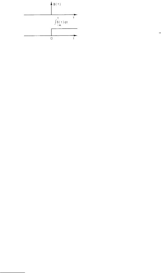
FIGURE 11.31. The δ function and its integral.
11.10 The Delta Function
It will be useful in the next sections to introduce a pulse that is very narrow, very tall, and has unit area under its curve. Physicists call this function the delta function δ(t). Engineers call it the impulse function u0(t).
The δ function is defined by the equations
11.11The Energy Spectrum of a Pulse and Parseval’s Theorem
For a |
signal |
with |
period T , |
|
the |
average |
power is |
|||||||||
|
1 |
T y2 |
(t)dt. We can also define the average power for |
|||||||||||||
T |
||||||||||||||||
0 |
|
|
|
|
|
|
|
|
|
|
|
|
|
|||
|
|
|
|
|
|
|
|
|
|
|
|
|
|
|
||
a signal lasting a very long time as |
|
|
|
|
||||||||||||
|
|
|
1 |
T |
|
2 |
|
2 |
1 |
2 |
|
2 |
|
|||
|
|
lim |
|
|
y |
|
(t)dt = a |
0 |
+ |
|
(a + b |
k |
). |
|||
|
|
|
|
|
|
|||||||||||
|
|
T →∞ 2T |
−T |
|
|
|
2 |
k |
|
|
||||||
|
|
|
|
|
|
k |
|
|
|
|||||||
|
δ(t) = 0, |
t = 0 |
|
|
∞ |
δ(t) dt = 1. |
(11.60) |
− |
δ(t) dt = |
|
|
−∞ |
|
|
The δ function can be thought of as a rectangle of width a and height 1/a in the limit a → 0, or as a Gaussian function (Appendix I) as σ → 0. Many other functions have the same limiting properties. The δ function is not like the usual function in mathematics because of its infinite discontinuity at the origin. It is one of a class of “generalized functions” whose properties have been rigorously developed by mathematicians6 since they were first used by the physicist P. A. M. Dirac.
Since integrating across the origin picks up this spike of unit area, the integral of the δ function is a step of unit height at the origin. The δ function and its integral are shown in Fig. 11.31. The δ function can be positioned at t = a by writing δ(t − a) because the argument vanishes at t = a.
Multiplying any function by the δ function and integrating picks out the value of the function when the argument of the δ function is zero:
∞ |
∞ |
y(t)δ(t) dt = y(0) |
δ(t) dt = y(0), |
−∞ |
−∞ |
∞ |
∞ |
y(t)δ(t − a) dt = y(a) |
δ(t − a) dt = y(a). |
−∞ |
−∞ |
(11.61) The second integral on each line is based on the fact that y(t) has a constant value when the δ function is nonzero so it can be taken outside the integral.
In the limit of infinite duration, both the integral and the denominator are infinite, but the ratio is finite.
For a pulse the integral is finite and the average power vanishes. In that case we use the integral without dividing by T . It is called the energy in the pulse.
Since y(t) is given by a Fourier integral, the energy in the pulse can be written as
∞ y2(t) dt = |
|
1 |
|
2 ∞ dt ∞ dω |
(11.63) |
|
|
2π |
|||||
−∞ |
|
−∞ |
−∞ |
|
||
|
|
|
|
|||
∞ |
dω [C(ω) cos ωt + S(ω) sin ωt] |
|||||
|
|
|||||
−∞ |
|
|
|
|||
× |
[C(ω ) cos ω t + S(ω ) sin ω t] . |
|||||
|
|
|
|
|
|
|
If the terms are multiplied out, this becomes |
|
|||||
∞ y2(t) dt = |
|
1 |
2 ∞ dt ∞ dω ∞ dω |
|||
|
||||||
−∞ |
|
2π |
−∞ |
−∞ |
−∞ |
|
|
|
|
||||
[C(ω) C(ω ) cos ωt cos ω t |
|
|||||
+ C(ω)S(ω ) cos ωt sin ω t |
(11.64) |
|||||
+S(ω)C(ω ) sin ωt cos ω t
+S(ω)S(ω ) sin ωt sin ω t] .
To simplify this expression, we interchange the order of integration, carrying out the time integration first. We assume that the function y(t) is su ciently well behaved so that this can be done.
Changing the order gives three integrals to consider:
∞
cos ωt cos ω t dt,
−∞
∞
cos ωt sin ω t dt,
−∞
∞
6A rigorous but relatively elementary mathematical treatment |
sin ωt sin ω t dt. |
is given by Lighthill (1958). |
−∞ |
11.12 The Autocorrelation of a Pulse and Its Relation to the Energy Spectrum |
305 |
These are analogous to the trigonometric integrals of Appendix E, except that they extend over all time instead of just one period. Therefore we might expect that an integral such as −∞∞ cos ωt sin ω t dt would vanish for all possible values of ω and ω . We might expect that the integrals −∞∞ cos ωt cos ω t dt and −∞∞ sin ωt sin ω t dt would vanish when ω =ω and be infinite when ω = ω . Such is indeed the case. This is reminiscent of the δ function, but it does not tell us the exact relationship of these integrals to it.
To find the exact values of the integrals we use the following trick. Let y(t) be the function for which C(ω) = δ(ω − ω ). Then, using Eqs. 11.55 and 11.61 we get
|
1.2 |
|
|
|
|
|
|
|
1.0 |
|
|
|
|
|
|
/(A/a)2 |
0.8 |
|
|
|
|
|
|
0.6 |
|
|
|
|
|
|
|
Φ′ |
0.4 |
|
|
|
|
|
|
|
|
|
|
|
|
|
|
|
0.2 |
|
|
|
|
|
|
|
0.0 |
|
|
|
|
|
|
|
-6 |
-4 |
-2 |
0 |
2 |
4 |
6 |
|
|
|
|
ω/a |
|
|
|
FIGURE 11.32. The energy spectrum Φ (ω) for an exponential pulse.
1 |
|
∞ |
1 |
|
||||
y(t) = |
|
|
δ(ω − ω ) cos ωt dω = |
|
cos ω t. |
|||
2π |
2π |
|||||||
|
|
|
−∞ |
|
|
|
||
The inverse equation for C(ω) is |
|
|
|
|||||
C(ω) = ∞ y(t) cos ωt dt = |
1 |
∞ cos ω t cos ωt dt. |
||||||
2π |
||||||||
−∞ |
|
−∞ |
|
|||||
But C(ω) = δ(ω − ω ). Therefore |
|
|
|
|||||
∞ |
|
|
|
|
|
|||
cos ωt cos ω t dt = 2π δ(ω − ω ). |
(11.65a) |
|||||||
−∞ |
|
|
|
|
|
|||
A similar argument shows that |
|
|
|
|||||
∞ |
|
|
|
|
|
|||
sin(ωt) sin(ω t) dt = 2π δ(ω − ω ). |
(11.65b) |
|||||||
−∞
The prime is to remind us that this is energy and not power. The left-hand side is the total energy in the signal, and y2(t) dt is the amount of energy between t and t + dt. This suggests that we call Φ (ω) dω/2π = Φ (f ) df the amount of energy in the angular frequency interval between ω and ω + dω or the frequency interval between f and f + df .
11.11.2 Example: The Exponential Pulse
The energy spectrum of the exponential pulse that was used earlier as an example is
A 2 |
1 |
|
||
Φ (ω) = C2(ω) + S2(ω) = |
|
|
|
. (11.68) |
a |
1 + (ω/a)2 |
|||
The fact that both the sine and cosine integrals are the same should not be surprising, since a sine curve is jut a cosine curve shifted along the axis and we are integrating from −∞ to ∞.
11.11.1Parseval’s Theorem
The integrals in Eqs. 11.65 can be used to evaluate Eq. 11.64. The result is
∞ 2 |
1 |
|
∞ |
∞ |
|||
y |
(t) dt = |
|
|
|
dω |
dω [C(ω)C(ω )δ(ω − ω ) |
|
2π |
|
||||||
−∞ |
|
|
|
−∞ |
−∞ |
||
|
+ S(ω)S(ω )δ(ω − w )] |
||||||
∞ y2(t) dt = |
|
1 |
∞ dω C2(ω) + S2(ω) . (11.66) |
||||
2π |
|||||||
−∞ |
|
|
−∞ |
|
|||
|
|
|
|
|
|||
This result is known as Parseval’s theorem. If we define the function
Φ (ω) = C2(ω) + S2(ω), |
(11.67a) |
||||
then Eq. 11.66 takes the form |
|
|
|||
∞ y2(t) dt = |
∞ Φ (ω) |
dω |
= ∞ Φ (f )df. |
(11.67b) |
|
2π |
|||||
−∞ |
−∞ |
−∞ |
|
||
|
|
||||
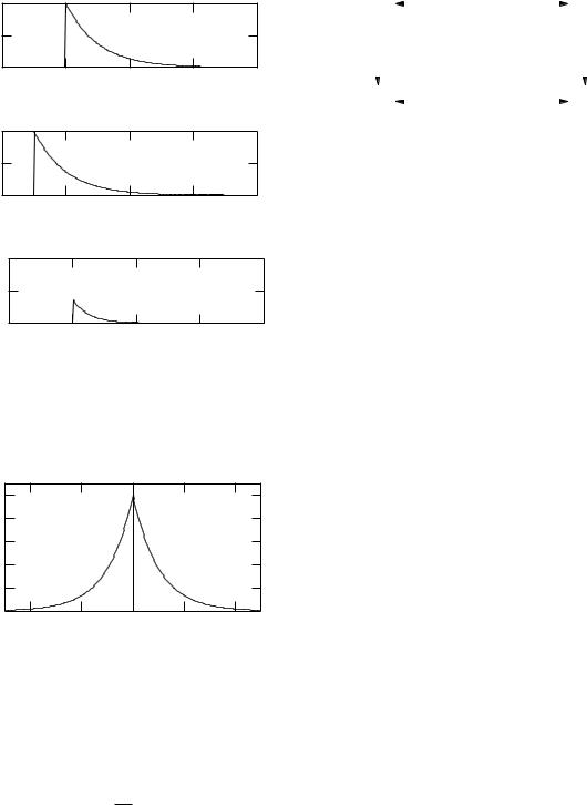
It is plotted in Fig. 11.32.
11.12The Autocorrelation of a Pulse and Its Relation to the Energy Spectrum
The correlation functions for pulses are defined as integrals instead of averages:
∞ |
|
φ12(τ ) = |
y1(t)y2(t + τ ) dt, |
−∞ |
(11.69) |
∞ |
|
φ11(τ ) = |
y1(t)y1(t + τ ) dt. |
−∞ |
|
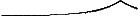
Consider the autocorrelation function of the exponential pulse, Eq. 11.58. Figure 11.33 shows the functions involved in calculating the autocorrelation for a typical positive value of τ . Since the autocorrelation function is even, negative values of τ need not be considered. The product of the function and the shifted function is (Ae−at)(Ae−a(t+τ )) = A2e−aτ e−2at. It can be seen from Fig. 11.33 that the limits of integration are from zero to
infinity. Thus, |
|
|
|
φ11(τ ) = A2e−aτ ∞ e−2at dt = |
A2e−aτ |
, τ > 0. |
|
2a |
|||
0 |
|
306 11. The Method of Least Squares and Signal Analysis
|
1.0 |
|
|
|
|
y(t) |
0.5 |
|
|
|
|
|
|
|
|
|
|
|
0.0 |
|
|
|
|
|
-2 |
0 |
2 |
4 |
6 |
|
|
|
t |
|
|
|
1.0 |
|
|
|
|
y(t+1) |
0.5 |
|
|
|
|
|
|
|
|
|
|
|
0.0 |
|
|
|
|
|
-2 |
0 |
2 |
4 |
6 |
|
|
|
t |
|
|
Product |
0.50 |
|
|
|
|
|
|
|
|
|
|
|
-2 |
0 |
2 |
4 |
6 |
|
|
|
t |
|
|
FIGURE 11.33. Calculation of the autocorrelation of the exponential pulse. The figure shows y(t), y(t + τ ), and their product, for τ = 1.
|
1.0 |
|
|
|
|
|
/2a) |
0.8 |
|
|
|
|
|
|
|
|
|
|
|
|
2 |
0.6 |
|
|
|
|
|
(τ)/(A |
|
|
|
|
|
|
0.4 |
|
|
|
|
|
|
11 |
|
|
|
|
|
|
|
|
|
|
|
|
|
φ |
0.2 |
|
|
|
|
|
|
|
|
|
|
|
|
|
0.0 |
|
|
|
|
|
|
-4 |
-2 |
0 |
2 |
aτ |
4 |
FIGURE 11.34. The autocorrelation function for an exponentially decaying pulse.
Because φ11 is even, the full autocorrelation function is
y (t) |
|
Fourier transform |
|
C(ω ), S(ω ) |
|||
|
|
|
|||||
|
|
||||||
Auto- |
|
|
|
|
|
|
Φ = C 2 + S 2 |
|
|
|
|
|
|
||
correlation |
|
|
|
|
|
|
|
φ |
|
(τ ) |
Fourier transform |
|
|
Energy |
|
|
|
|
|||||
|
|
|
Φ (ω ) spectrum |
||||
|
|
||||||
11 |
|
|
|
|
(continuous) |
||
|
|
|
|
|
|
|
|
FIGURE 11.35. Two ways to obtain the energy spectrum of a pulse signal.
We have seen this integral before, in conjunction with Eq. 11.59. The result is
A 2 |
1 |
|
||
Φ (ω) = |
|
|
|
. |
a |
1 + (ω/a)2 |
|||
Comparing this with Eq. 11.67, we again see that
Φ (ω) = C2(ω) + S2(ω). |
(11.71) |
This relationship between the autocorrelation and Φ can be proved in general by representing each function in the definition of the autocorrelation function by its Fourier transform, using the trigonometric addition formulas, carrying out the time integration first, and using the δ-function definitions. The result is
φ11(τ ) = |
1 |
∞ C2(ω) + S2(ω) cos ωτ dω |
||
2π |
||||
|
−∞ |
|
||
|
|
|
||
= |
1 |
∞ Φ (ω) cos ωτ dω. |
(11.72) |
|
2π |
||||
|
−∞ |
|
||
As with the periodic signal, there are two ways to go from the signal to the energy spectrum. The Fourier transform is taken of either the original function or the autocorrelation function. Squaring and adding is done either in the time domain to y(t) to obtain the autocorrelation function, or in the frequency domain by squaring and adding the coe cients. The Fourier transforms can be taken in either direction. Squaring and adding is onedirectional and makes it impossible to go from the energy spectrum back to the original function. These processes are illustrated in Fig. 11.35.
φ11(τ ) = |
A2 |
(11.70) |
2a e−a|τ |. |
This is plotted in Fig. 11.34.
The autocorrelation function has a Fourier transform Φ . Only the cosine term appears, since φ11 is even:
Φ (ω) = |
A2 |
∞ a t |
| cos ωt dt |
|
|
−∞ e− | |
|||
2a |
||||
= |
A2 |
∞ e−at cos ωt dt. |
||
a |
||||
|
0 |
|
||
11.13 Noise
The function y(t) we wish to study is often the result of a measurement of some system: the electrocardiogram, the electroencephalogram, blood flow, etc., and is called a signal. Most signals are accompanied by noise. Random noise fluctuates in such a way that we cannot predict what its value will be at some future time. Instead we must talk about the probability that the noise has a certain value. A key problem is to learn as much as one can about a signal that is contaminated by noise. The techniques discussed in this chapter are often useful.