Intermediate Physics for Medicine and Biology - Russell K. Hobbie & Bradley J. Roth

This can be multiplied by 2πr dr and integrated over the pore area. There are two integrals to consider. The first defines the average current density for a particular species:

The second defines an e ective di usion constant:

Rp

0

The integrated current density equation is

Consideration of the r dependence in the pore has given an equation exactly like Eq. 9.42, but with De instead of D. Equations 9.43 and 9.44 are still valid. The form of λ is unchanged: λ = −kB T L/zev. Conversion from a single pore to unit area of the membrane requires multiplying j by nπRp2. We define ωsRT = nπRp2De /L and call the concentration outside C1 and the concentration inside C2. The electric current density per unit area of membrane is

Suppose that three species can pass through the membrane: sodium, potassium, and chloride. Equation 9.54 can be applied separately to each species to obtain the

GHK current equation for each ion species:

As an example of the use of the GHK voltage equation, consider how the reversal potential depends on the concentration of some external ion. We will use the concentrations of Fig. 6.2, except for the ion whose concentration is being changed. The particle concentrations are in mmol l−1 (any units can be used since ratios are taken):

The permeabilities are not known. However, only the ratio to ωK matters. If we take the ratio ωK : ωNa : ωCl to be 1.0 : 0.04 : 0.45 and use T = 300 K, then Eq. 9.56 is (in mV)

This has been plotted in Fig. 9.11 for variations of [K1] and [Na1]. In each case Cl ions are also added to the external solution in an equal amount. There is a region of potassium concentration over which the behavior is nearly exponential, and one could be misled into thinking that the potential–concentration relation was given either by the Nernst equation alone or by Donnan equilibrium. The potential change with sodium concentration is much less because of the low permeability of the membrane to sodium.

The assumption that the total current through the membrane is zero guarantees that there will be no charge buildup inside the cell; however, the individual currents are not zero, so there may be concentration changes with time. We will next investigate the magnitude of this effect. Equation 9.54 can be converted to particle flux instead of charge flux by dividing by ze. The result for ion

The reversal potential, vrev, is the potential for which the total membrane current or fluence rate, that is the sum of the three fluence rates, is zero. The amount of charge within the cell does not change with time, but the concentration of each species within the cell changes with time. This less stringent requirement becomes JNa + JK + JCl = 0. Adding Eqs. 9.55 together and factoring out NAe2v/(1 − e−ev/kB T ) gives

(ωNa [Na1] + ωK [K1] + ωCl [Cl2]) e−ev/kB T = ωNa [Na2] + ωK [K2] + ωCl [Cl1] ,

or the GHK voltage equation

FIGURE 9.11. The potential di erence across a cell membrane as a function of changes in the exterior concentration of KCl or NaCl, calculated using the Goldman equation.

238 9. Electricity and Magnetism at the Cellular Level

s is

C e−zev/kB T − C

1 2

Js = zevωs 1 − e−zev/kB T .

The concentrations are converted from mmol l−1 to particles m−3 by multiplying by Avogadro’s number. (The factors of 103 in the conversion happen to cancel out.) Consider the previous example at T = 300 K, [K1] = 5, [Na1] = 145, and v = −68.17 mV. The exponential factor for the positive ions is e−ev/kB T = 13.929, while for the chloride ion it is the reciprocal, 0.0718. If we write ωNa = 0.04ωK and ωCl = 0.45ωK, then the fluxes for the three ions are

JK = +(6.55 × 103)ωK(6.215),

JNa = −(6.55 × 103)ωK(6.202),

JCl = −(6.55 × 103)ωK(0.013),

and the total current is zero.

Although the GHK equations are widely used because of their simplicity, some cautions are in order. Their derivation assumed independence of the moving ions. We know that this is an oversimplification for several reasons. Experiments show that the currents saturate for high concentrations. The distortion of the electric field by other ions was ignored. The permeability (di usion constant) was assumed to be constant. The pore was assumed to have a constant cross section and constant electric field. A somewhat less restrictive model for the reversal potential (the potential at which the current density becomes zero and changes sign) can be derived for a pair of ions with the same valence if we assume that any variations in D(x) for the two ions are similar (Problem 18). With that assumption the reversal potential is

When ions have di erent valences, the GHK equation becomes more complicated. Lewis (1979) has derived an analogous equation for transport of sodium, potassium and calcium.

9.7 Membrane Channels

In Chapter, 6 we described some of the properties of the sodium and potassium channels in a squid axon. There are many other kinds of channels. Variations exist not only from one organism to another, but in di erent kinds of cells in the same organism. The classic monograph on ionic channels is the book by Hille (2001).

There are several di erent kinds of potassium channels. Most open after depolarization; a few open after hyperpolarization. Potassium channels in axons (such as the ones we encountered in Chapter 6) are called delayed rectifiers because of their delay in opening after a voltage step.

The properties of sodium channels are more uniform from one cell type to another.

Calcium channels pass much smaller currents than sodium or potassium channels because calcium concentrations are much smaller; the calcium current density is usually about 101 the current density for sodium or potassium. Calcium channels typically activate with depolarization. Since the concentration of calcium inside cells is usually very small, the interior calcium concentration can increase 20-fold in response to depolarization. This increase in concentration can initiate a chemical reaction, for example, to cause contraction of a muscle cell.

Chloride channels often have a large conductivity. The chloride concentration ratio in some muscle cells is such that the resting potential is close to the chloride Nernst potential. As a result, small changes in the potential cause relatively large chloride currents, which tend to stabilize the resting potential.

The earliest voltage-clamp measurements were di cult to sort out. Hodgkin and Huxley changed the concentration of extracellular sodium, substituting impermeant choline ions, to determine what part of the current was due to sodium and what was due to potassium. Figure 9.12(a) shows typical currents.

In the mid-1960s, various drugs were found that at very small concentrations selectively block conduction of a particular ion species. We now know that these drugs bind to the channels that conduct the ions. An example is tetrodotoxin (TTX), which binds to sodium channels and blocks them, making it a deadly poison.

The next big advance was patch-clamp recording [Neher and Sakmann (1976)]. Micropipettes were sealed against a cell membrane that had been cleaned of connective tissue by treatment with enzymes. A very-high- resistance seal resulted [(2–3)×107 Ω] that allowed one to see the opening and closing of individual channels. For this work Erwin Neher and Bert Sakmann received the Nobel Prize in Physiology or Medicine in 1991. Around 1980, Neher’s group found a way to make even higherresistance (1010–1011 Ω) seals that reduced the noise even further and allowed patches of membrane to be torn from the cell while adhering to the pipette [Hamill et al. (1981)]. The relationship of noise to resistance will be discussed below.

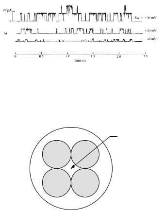
The patch-clamp studies revealed that the pores open and close randomly, as shown in Fig. 9.13. Thus, the Hodgkin–Huxley model describes the average behavior of many pores, not the kinetics of single pores. Note how the current through an open pore changes as a function of the applied potential. A single open pore can pass at least 1 pA of current or 6 × 106 monovalent ions per second. Most can pass much more. While no perfectly selective channel is known, most channels are quite selective: for example, some potassium channels show a 100:1 preference for potassium over sodium.

Gene splicing combined with patch-clamp recording provided a wealth of information. Regions of the DNA

j, mA cm-2

6

Steady-state potassium current

4

2

0

Peak sodium current

-2 -40 0 40 80

Clamp potential, mV

(a)

10

0 -40 0 40 80

Clamp potential, mV

(b)

responsible for synthesizing the membrane channel have been identified. One example that has been extensively studied is a potassium channel from the fruit fly,

Drosophila melanogaster. The Shaker fruit fly mutant shakes its legs under anesthesia. It was possible to identify exactly the portion of the fly’s DNA responsible for the mutation. When Shaker DNA was placed in other cells that do not normally have potassium channels, they immediately made functioning channels.

The current view is that the Shaker potassium channel consists of four subunits that span the membrane. The pore presumably runs along the fourfold-symmetry

axis, as shown in end view in Fig. 9.14. Sodium and calcium channels are very similar. Voltage-gated channels are reviewed by Sigworth (1993) and by Keynes (1994).

Recently, MacKinnon and his colleagues determined the three-dimensional structure of a potassium channel using X-ray di raction [Doyle et al. (1998); Jiang et al. (2003)]. The channel protein contains four identical subunits, arranged with fourfold symmetry around a central pore (Fig. 9.14). Each subunit has two alpha helices that cross the membrane and an inner pore region. One of the remarkable features of this channel is that potassium ions are 10,000 times more likely to pass through than sodium

240 9. Electricity and Magnetism at the Cellular Level

FIGURE 9.13. Opening of single K(Ca) channels. From B. S. Pallotta, K. L. Magleby, and J. N. Barrett (1981). Single channel recordings of Ca2+-activated currents in rat muscle cell culture. Nature 293: 471–474. Reprinted with permission from Nature (London).

Pore

FIGURE 9.14. Current understanding of the structure of a Shaker potassium channel. There are four subunits that traverse the membrane and create a pore at their center.

ions. Yet, potassium and sodium have similar chemistry (they are in the same column of the Periodic Table), and their ions are identical except for size (0.133 nm radius for potassium, 0.095 nm for sodium).

The channel structure suggests that a narrow, 1.2 nm long region of the pore is responsible for selectivity. As the ion enters this region, there is not enough room for the polar water molecules that normally surround it and shield its charge. Instead, carbonyl oxygen atoms on the channel protein come in close contact with the potassium ion and provide the shielding. The size of the pore is such that potassium ions fit snugly with the surrounding carbonyl oxygen atoms, but sodium does not fit as well.

X-ray di raction studies have also clarified the mechanism of voltage dependence in potassium channels. The pore is surrounded by charged structures on the channel’s perimeter that sense the transmembrane voltage. These structures act somewhat like levers, opening and closing the pore in response to the voltage. The movement of these structures is responsible for gating currents in these channels. Roderick MacKinnon received the 2003 Nobel Prize in Chemistry for this work on the potassium channel.

Let us now explore some of the physics of channels. Combining the macroscopic current density with the current in a single channel shows that there are not many channels per unit area of the membrane (see Problems 19 and 20). It is illuminating to consider what e ect currents of this magnitude and duration have on the transmembrane potential. The capacitance per unit area of biological membranes is about 0.01 F m−2 (1 µF cm−2). A channel conducting 1 pA for 1 ms allows 10−15 C to pass. This is enough charge to change the potential 100 mV on an area of 10−12 m2 or 1 µm2. This charge transfer corresponds to about 6,000 monovalent ions per µm2.

Figure 9.12(a) shows the steady-state potassium and peak sodium current densities for a squid axon. The ion concentrations are known, and we saw in Chapter 6 that the Nernst potentials at 6.3 ◦C were +50 mV for sodium and −77 mV for potassium. Figure 9.12(b) shows the conductance per unit area, obtained by dividing the current by v − vNernst. Figure 9.12(c) shows a semilogarithmic plot of the conductance per unit area.

The sodium current density changes sign at the sodium Nernst potential. While a measured zero crossing is an accurate way to determine the Nernst potential, extrapolation to find the zero-crossing can be quite misleading. The potassium current density appears to be linear over a large region, and it is tempting to extrapolate to find vK. The extrapolation shows zero current at about −40 mV, which is far from vK. The reason can be seen in Fig. 9.12(b), which shows that gK is varying considerably over the region where jK appears to be linear; this distorts the slope and changes the extrapolated intersection.

A simple two-state model can explain the shape of the curves in Fig. 9.12(c). The conductance per unit area of a membrane is the product of the conductance of an open pore and the average number of pores per unit area that are open. The model assumes that each channel has a gate that is either open or closed. When the gate is open, the channel has a conductance determined by the passive properties of the rest of the channel. The rapid increase of conductance between −60 and −30 mV corresponds to a rapidly increasing probability that the gate is open.

Suppose that each channel has a gate with two states: open and closed. When there is no average electric field in the membrane (v = 0) the energy of the open state is w = uokB T greater than the closed state. Suppose also that as the gate opens and closes, a charge q associated with the gate moves a small distance parallel to the axis of the pore. When there is a potential v across the membrane, the charge moves through a potential difference αv, where α < 1. The total energy change when the gate opens with potential v across the membrane is then w + qαv. The quantity qα is often written as ze and called the equivalent gating charge. In terms of kB T the energy change when the pore opens is u = uo + zev/kB T .

Let po be the probability that a pore is open and pc be the probability that it is closed. The probabilities are related by a Boltzmann factor: po = pce−u. Since

Clamp potential, mV

FIGURE 9.15. Plot of sodium and potassium conductivities from Fig. 9.12(c) with fits by Eq. 9.58. For sodium uo = −10.5 and z = −7; for potassium uo = −19 and z = −10.

po + pc = 1, po = e−u/(1 + e−u) = 1/(1 + eu),

For very large values of u (small values of po),

FIGURE 9.16. The results of a set of experiments with Shaker potassium channels. Panel A shows the macroscopic depolarizations to +20 and +80 mV for a patch with about 400 channels. Panel B shows the gating current recorded from another patch containing about 8,000 channels. Potassium was removed from the solution bathing the interior surface of the membrane. Panels C and D show recordings similar to panel A, but with many fewer channels in the patch. The results from three successive depolarizing pulses are shown in each case. From F. J. Sigworth (1993). Voltage gating of ion channels. Quart. Rev. Biophys. 27: 1–40. Reprinted with permission of Cambridge University Press.

242 9. Electricity and Magnetism at the Cellular Level

current of 1 pA is 6.25 ×106 monovalent ions per second, so that the average time between the passage of successive ions through the channel is 1.6×10−7 s. In a uniform electric field giving 80 mV across the membrane, a monovalent ion would have a drift velocity of 0.6 m s−1 based on the bulk di usion constant. [See the discussion surrounding Eq. 4.22.] Because ions in the pore are confined,

let us use 101 of this, or 0.06 m s−1. (The di usion constant is proportional to the solute permeability; see Sec.

5.9. Ignoring electric forces, we see from Fig. 5.19 that ω/ω0 = 0.1 corresponds to a/Rp = 0.4. So this is probably still a high drift velocity.) Then the time it takes the ion to pass through the channel is its length (assume 6 nm) divided by the average speed, or 10−7 s. The fraction of the time there is an ion in the channel is f = 0.625.

We can make some other estimates of channel parameters. Over some part of its length, the channel must be narrow enough so the wall can interact directly with the ion that is passing through, not shielded by water molecules. The pore must therefore narrow to a radius of 0.3 to 0.7 nm in some region. Let us assume a cylindrical pore of radius a = 0.7 nm and length h = 6 nm. The average number of water molecules in the channel is 308; the average concentration of ions is f /(πa2h) = 113 mmol l−1, which is about right. The resistance of a channel while it is open is R = v/i = 80 mV/1 pA = 8 × 107 Ω. (We should actually use v − vNernst, but this is a rough estimate. If we were going to be more accurate, we should also use the Nernst–Planck equation, recognizing that the ions move by di usion as well as drift.)

9.8 Noise

The current fluctuates while a channel is open, as can be seen in Figs. 9.13 and 9.16. Some of the fluctuation is due to noise in the measurement apparatus. However, there are some fundamental physical lower limits to the fluctuations resulting from noise in the membrane patch itself. We discuss these briefly here, with a more extensive discussion in Chapter 11. DeFelice (1981) wrote an excellent book on noise in membranes.

9.8.1 Shot Noise

Poisson limit of the binomial distribution (Appendix J). The variance in the number of ions is σn2 = n = i∆t/e. Since the average charge transported is q = ne, the variance in the charge is σq2 = e2σn2 = ei∆t. When many samples of length ∆t are measured, the variance in the current is σi2 = σq2/(∆t)2. The standard deviations are

and the fractional standard deviations are

For a current of 1 pA, the fractional standard deviation is 0.013 when the sampling time is 1 ms and 0.04 when the sampling time is 0.1 ms. These are much smaller than what is observed in the figures.

9.8.2 Johnson Noise

The next source of noise is called Johnson noise. It arises from thermal fluctuations or Brownian movement of the ions. It can be derived from a microscopic model of conduction (either in an ionic solution or a metal), but we will do it using the equipartition of energy.

First, we need an expression for the energy U contained in a charged capacitor. To obtain it, imagine that an amount of charge +dq is transferred from the negative to the positive conductor. This increases the amount of positive charge on the positive conductor and also increases the amount of negative charge on the negative conductor. The work required to transfer the charge when the potential di erence between the conductors is v is vdq. The energy stored in the capacitor is the total work required to charge the conductor from 0 to q. Remembering that q = Cv, we have

The first (and smallest) limitation is called shot noise. It is due to the fact that the charge is transported by ions that move randomly and independently through the channels. Imagine a single open conducting channel with an average current i of monovalent ions. During time ∆t (which can be any interval shorter than the time the channel is open) the average charge flow is i∆t and the average number of ions is n = i∆t/e. Since there are a very large number of ions that might flow through the channel (occurrences) and the probability that any one ion moves through the channel during ∆t is very small, we have the

If the capacitor is completely isolated, there can be a constant charge on each conductor with no fluctuations. If the capacitor is in thermal contact with its surroundings and is in equilibrium, then the equipartition theorem applies. The capacitor can be brought into thermal equilibrium with its surroundings by connecting a resistance R between the conductors. This will discharge the capacitor so q = v = 0. There will be fluctuations around these zero values. Because the expression for the energy depends on the square of the variables, the mean square value is given by the equipartition of energy theorem,

Eq. 3.38. We will assume that when the capacitor is charged, thermal fluctuations give the same variances as when it is discharged:

Since changes in current or voltage in an RC circuit occur with time constant τ = RC, we can also write these as

These are special cases of a more general relationship that will be discussed in Chapter 11.

We can use these to determine some of the requirements for patch-clamp recording. In order to see the current from a single channel with some accuracy, let us require that the standard deviation of the current fluctuation be less than 18 of the signal we want to measure. (This signal-to-noise ratio, SNR, of 8 is arbitrary.) First consider the limitation due to Johnson noise. We want σi < i/8 or σi2 < i 2 /64. From this we obtain

The capacitance of a patch of membrane of 1 µm radius is 3.1 × 10−14 F. At a temperature of 300 K and for an average current of 1 pA, this gives R > 3 ×109 Ω. Larger values of R will give an even higher SNR. There are several sources of thermal noise in a recording electrode, all discussed in the paper by Hamill et al. (1981). These are order-of-magnitude results; one must determine carefully which capacitances and resistances provide the dominant e ects.

We can also see when shot noise is important. The ratio of Johnson noise to shot noise is

This ratio is less than 1 and shot noise is important when R > kB T /ei = 2.6 ×1010 Ω. Shot noise has been detected in channel gating currents and subjected to very sophisticated analysis. See the paper by Crouzy and Sigworth (1993) and the references therein.

9.9 Sensory Transducers

Animals have very sensitive senses. We will see (Problem 13.19) that the ear can hear sounds at 1,000 Hz that are just greater than the pressure fluctuations due

Ion

Channel

Hair Cell

FIGURE 9.17. A schematic diagram of two stereocilia linked by a filament that opens a channel as the cillia move back and forth.

to molecular collisions on the ear drum. An eye that is adapted to the dark can detect flashes of light corresponding to a few photons (Chapter 14). Many animals can smell chemicals when only a few molecules strike their sensory organs. The electric skate can detect extremely small electric fields.

In each case a transducer converts the sensory stimulus into a series of nerve impulses. The transducer must have su cient sensitivity to respond to the stimulus, and it must also absorb an amount of energy from the stimulus that is greater than what it receives from random thermal bombardment (Brownian movement).5 We describe here two transducers: the mechanoreceptors (hair cells) of the inner ear and the electric organ of the skate.

Various transduction mechanisms are reviewed in Chapter 8 of Hille (2001). The mechanoreceptors of the bullfrog inner ear have been studied for many years. The hair-cell current rises from 0 to 100 pA with an 0.5-µm displacement. Each hair cell is cylindrical. On its end face are found about 60 very small stereocilia, each 1–50 µm long and with a 100–500-nm radius. The tips of these stereocilia are linked by thin filaments. The hair cell and stereocilia that detect sound in the ear are attached to the basilar membrane in the cochlea of the ear and move in a very viscous fluid as the basilar membrane vibrates. Hair cells detecting accelerations of the entire animal are attached to a suspended dense body. It is believed that as the stereocilia move, these filaments pull open flaps at the end of ion channels, allowing ions to enter the cell and initiate the conduction process. This is shown schematically in Fig. 9.17. Denk and Webb (1989) have used a laser interferometer to measure the motion of the hair cells. They found that the spontaneous motion consists primarily of thermal excitation (Brownian motion). Fluctuations in the intracellular voltage were also measured. They often correlated with the motion of the hair cells.

Freshwater catfish respond to electric fields as low as 10−4 V m−1. Saltwater sharks and rays can detect fields of 5 × 10−7 V m−1. A brief review has been given by Bastian (1994); Kalmijn (1988) provides a very complete

5For the detection of light, the amount of energy per photon is so much greater than kB T that shot noise dominates.

244 9. Electricity and Magnetism at the Cellular Level

review. The saltwater fish have a more complicated sensory apparatus than the freshwater fish, known as the ampullae of Lorenzini. Kalmijn and his colleagues discovered that the ocean flounder generates a current dipole of 3 ×10−7 A m. In sea water of resistivity 0.23 Ω m this gives an electric field of 2 × 10−5 V m−1 at a distance 10 cm in front of the flounder. They were able to show in a beautiful series of behavioral experiments that dogfish (a small shark) could detect the electric field 0.4 m from a current dipole of 4 × 10−7 A m, corresponding to an electric field of 5 × 10−7 V m−1. The fish would bite at the electrodes, ignoring a nearby odor source. A field of 10−4 V m−1 would elicit the startle response. A field 101 as large caused a physiologic response. The animals responded to a constant field or a sinusoidally alternating field up to 4 Hz. At 8 Hz the threshold increased by a factor of 2.

In a series of experiments, Lu and Fishman (1994) dissected out the ampulla of Lorenzini and measured its response in the laboratory. They found that the resting rate of firing of the organ is about 35 Hz (impulses per second) and that an applied electric potential increases or decreases the firing rate by about 1 Hz µV−1, depending on its sign. The firing rate saturated for potential di erences of 100 µV.

The behavioral experiments showed sensitivity to an electric field of 0.5 µV m−1. The anatomy of the ampulla is such that the organ senses the potential di erence between the surface of the fish and deep in its interior. Pickard (1988) shows that for a spherical fish of radius a, this gives a potential of 3aE/2, where E is the external electric field. The amplitude of the potential di erence oscillation of a fish of length 13 m is therefore 0.25 µV. This is enough to cause a 1% change in firing rate, which could be detected by neuronal circuits [Adair et al. (1998)].

The Johnson noise is somewhat smaller than the signal detected. To estimate it, use Eq. 9.63a with the ampullary capacitance of 0.15 µF measured by Lu and Fishman. The standard deviation of the noise is 0.17 µV.

9.10Possible E ects of Weak External Electric and Magnetic Fields

9.10.1 Introduction

There is a lingering controversy over whether radiofrequency and power-line-frequency (50–60 Hz) electric or magnetic fields can cause cancer. While the e ect, if any, is quite small, the literature is extensive, involving both epidemiological and laboratory studies. Results are conflicting, and the mechanisms by which such an e ect might occur are not yet understood. Mechanisms have been proposed, some of which are inconsistent with basic physical principles such as the Boltzmann factor, the mean free path of ions, and thermal fluctuations. It is be-

yond our scope to do more than provide pointers to the field and discuss some basic underlying physics.

A review in the physics-teaching literature was provided by Hafemeister (1996). An excellent discussion of the all aspects of the problem is available at a frequently updated website, Powerlines and Cancer FAQ [Moulder (Web)]. Similar websites for cell phones and for static fields can be reached through this one.

We have seen that electric charges give rise to electric fields, and moving electric charges (currents) generate magnetic fields. The electric field lines start and end on charges, and the magnetic field lines surround the currents. We will see in Chapter 14 that accelerated charges generate electromagnetic radiation, in which the electric and magnetic fields are interrelated and the field lines close on themselves far from the source charges. Energy is radiated: it leaves the source and never returns. This radiated energy is in the form of discrete packets or photons, whose energy is related to the frequency of oscillation of the fields. The energy of each photon is E = hν, where h is Planck’s constant and ν the frequency. At room temperature, the energy of random thermal motion is kB T = 4×10−21 J. At 60 Hz, the energy in each photon is much smaller: 4 × 10−32 J. At 100 MHz it is 7 × 10−26 J. For electromagnetic radiation in the ultraviolet and beyond, which certainly can harm cells, the photon energy is 5 × 10−19 J or greater, quite large compared to kB T . At the very low frequencies we are considering, it is the strength of the electric or magnetic field that is important, not the energy of individual photons. A more detailed discussion of the distinction between these lowfrequency “near fields” and “radiation fields” is found in Polk (1996).

9.10.2E ects of Strong Fields

We have seen electrical burns, cardiac pacing, and nerve and muscle stimulation produced by electric or rapidly changing magnetic fields. Even stronger electric fields increase membrane permeability. This is believed to be due to the transient formation of pores (electroporation). Pores can be formed, for example, by microsecond-length pulses with a field strength in the membrane of about 108 V m−1 [Weaver (2000)]. Microwaves are used to heat tissue. Nerve stimulation requires a few millivolts across the cell membrane, or about 105–106 V m−1. Both electric and magnetic fields are used to promote bone healing, with field strengths in tissue in the fracture region of 10−1 V m−1 [Tenforde (1995)], though these results are still controversial [Adair (2000)].

9.10.3Fields in Homes are Weak

Much weaker fields in homes are produced by power lines, house wiring, and electrical appliances. Barnes (1995) found average electric fields in air next to the body of about 7 V m−1, with peak values of 200 V m−1. (We will

find that since the body is a conductor, the fields within the body are much less.) Average residential magnetic fields are about 0.1 µT, with peaks up to four times as large. Within the body they are about the same. Tenforde (1995) reviews both power-line- and radio-frequency field intensities.

9.10.4 Epidemiological Studies

Epidemiological studies have been very valuable in tracing the cause of infectious outbreaks. They have also indicated that smoking increases the probability of developing lung cancer by 3,000%—a factor of 30. However, there are di culties with epidemiological studies when the effect is small: there are inescapable statistical fluctuations unless the number of subjects is huge; associations do not prove causality; and there may be unrecognized variables that are confusing the picture. The problem is exacerbated when positive findings receive widespread publicity and negative findings are ignored by the press.

Epidemiological studies usually report “relative risk:” the incidence in an exposed group divided by the incidence in an unexposed group. A relative risk of one means no e ect. Moulder (Web, question 20A) says,

A strong association is one with a relative risk (RR) of 5 or more. Tobacco smoking, for example, shows a strong association, with the risk of lung cancer in smokers being 10-30 times that of nonsmokers. A relative risk of less than about 3 indicates a weak association. A relative risk below about 1.5 is essentially meaningless unless it is supported by other data.

Most of the positive power-frequency studies have relative risks of 2 or less. The leukemia studies as a group have relative risks of 0.8-1.9, while the brain cancer studies as a group have relative risks of 0.8-1.6. This is a weak association. Interestingly, as the sophistication of the studies has increased, the relative risks have not increased.

One would also expect an increased response with increasing dose. Moulder continues,

9.10.5 Laboratory Studies

The many laboratory studies are also reviewed by Moulder (Web). He concludes:

Power-frequency fields show little evidence of the type of e ects on cells, tissues or animals that point towards their being a cause of cancer, or to their contributing to cancer. In fact, the existing laboratory data provides strong evidence that power-frequency fields of the magnitude to which people are exposed are not carcinogenic.6

9.10.6Reviews and Panel Reports

Moulder (Web) lists a number of review articles and reports by expert panels. We note only a few here. Reviews by Moulder and Foster (1995, 1999) find that the association between power-frequency fields and cancer is weak7 for magnetic fields and even weaker for electric fields. Carstensen (1995) and Bren (1995) reach similar conclusions.

A report by a committee of the National Research Council concludes that

the current body of evidence does not show that exposure to these fields presents a humanhealth hazard.... The committee reviewed residential exposure levels to electric and magnetic fields, evaluated the available epidemiological studies, and examined laboratory investigations that used cells, isolated tissues, and animals.” [National Research Council (1997), p. 2]

There is no convincing evidence that exposure to 60-Hz electric and magnetic fields causes cancer in animals.... There is no evidence of any adverse e ects on reproduction or development in animals, particularly mammals, from exposure to power-frequency 50or 60-Hz electric or magnetic fields.” [National Research Council (1997), p. 7].

No published power-frequency exposure study has shown a statistically significant dose– response relationship between measured fields and cancer rates, or between distances from transmission lines and cancer rates. However, there is some indication of a dose-response in some of the older childhood leukemia studies when wire codes or calculations of historic fields are used as exposure metrics. The lack of a clear relationship between exposure and increased cancer incidence is a major reason why most scientists are skeptical about the significance of much of the epidemiology.

6Foster (1996) has reviewed many of the laboratory studies and describes cases where subtle cues meant the observers were not making truly “blind” observations. Though not directly relevant to the issue under discussion here, a classic study by Tucker and Schmitt (1978) at the University of Minnesota is worth noting. They were seeking to detect possible human perception of 60-Hz magnetic fields. There appeared to be an e ect. For 5 years, they kept providing better and better isolation of the subject from subtle auditory clues. With their final isolation chamber, none of the 200 subjects could reliably perceive whether the field was on or o . Had they been less thorough and persistent, they would have reported a positive e ect that does not exist.

7That is, the carcinogenic e ects are in International Association for Research on Cancer group 2B (possibly carcinogenic), a group that includes co ee and pickled vegetables [Moulder (Web) Q. 27F].

246 9. Electricity and Magnetism at the Cellular Level

FIGURE 9.18. An infinite slab of tissue is immersed in an oscillating electric field of amplitude E0 in air.

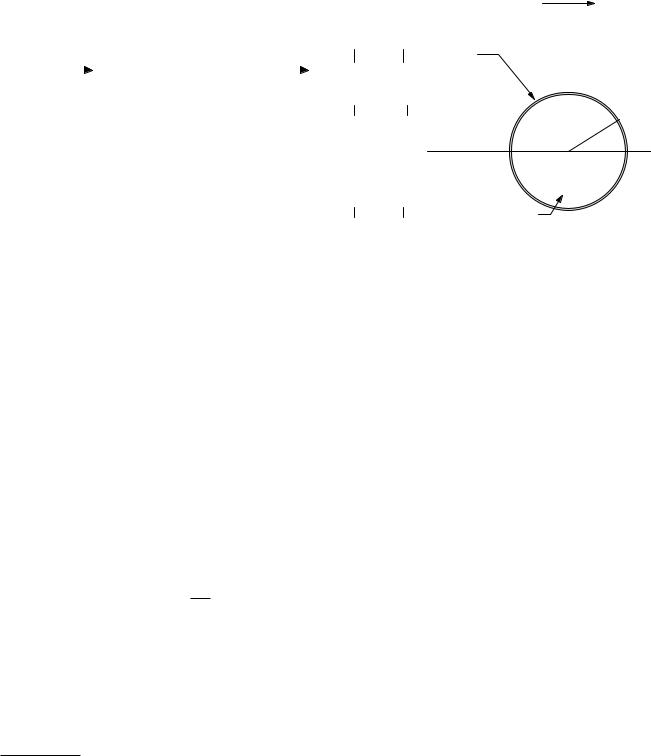
E1

(far away)

E just outside = (3 / 2)E1 sinθ

E in membrane = (3 / 2)(a /b)E1 cos θ

θ

E intracellular = (3 / 2)(a /b)(σ membrane /σ )E1

9.10.7 Electric Fields in the Body

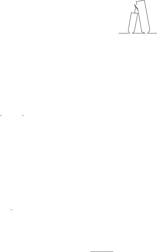
We now review some of the basic principles that govern the interaction of electric and magnetic fields with the body. One of the important principles is the relationship between the electric field in air and the field within the body, which is a conductor. A simple model that shows how this coupling takes place is the one-dimensional problem shown in Fig. 9.18.

An infinite slab of tissue has dielectric constant κ and conductivity σ. In the air perpendicular to the surface of the slab is an external oscillating electric field E(t) = E0 cos ωt. We assume that the dielectric constant is independent of frequency and accounts for the polarization of the tissue. An ionic current flows and causes free charge per unit area ±σq to accumulate on the surfaces of the slab. Within the slab the field is E1(t) and the current density is j = σE1. Gauss’s law (Eq. 6.21b) applied to either surface gives

Conservation of free charge at the surface requires that8

If we di erentiate Eq. 9.67 and combine it with Eq. 9.68, we obtain

The factor κ 0/σ is characteristic of the tissue and has the dimensions of time. We will call it τt.9 Typical tissue conductivity is about 0.1 S m−1. We must be careful

8Readers who are familiar with the concepts of reactance and complex impedance must be frustrated because we have not used them. The reason is pedagogic. Because many in our intended audience may have had only one year of calculus, we want to avoid the use of complex numbers. In Chapter 11 we introduce them as a parallel notation. They are widely used in the image reconstruction described in Chapter 12.

9Recall that the membrane time constant τ , was used in Eq. 6.40. The values of conductivity or resistivity and dielectric constant are di erent in this case.

FIGURE 9.19. The electric fields in and around a spherical cell. The cell has radius a and membrane thickness b. The field far from the cell has amplitude E1.

about the value of the dielectric constant. We have used a value of 80 for water. However, tissue is much more complex than pure water and there are several e ects that alter the dielectric constant [Foster and Schwan (1996)]. It takes time for both the polarization charges and conducting ions to move. As a result, both the conductivity and the dielectric constant of tissue depend on the frequency of the applied electric field and in fact are not independent of one another [see Foster and Schwan (1996), especially pp. 31–41].

Several e ects change the conductivity and dielectric constant as a function of frequency. At power-line frequencies the dominant e ect is the slight movement of the counterions and charge in the double layer at a cell membrane in response to the applied electric field. As a result, κ ≈ 106 and τt = 9.1 × 10−5 s.

We try a solution to Eq. 9.69 of the form E1(t) = A sin ωt + B cos ωt. It satisfies the equation if

For 60 Hz and a dielectric constant of 106, A = 33 × 10−9E0, B = 1.1 ×10−9E0. The amplitude of the field in tissue is E1 ≈ A. The field in air is reduced by a factor of about 3 × 10−8 in tissue because the tissue is a good conductor. The total reduction is nearly the same for a dielectric constant of 80, as can be seen from the fact that the approximate form for A does not depend on κ.

9.10.8 Electric Fields in a Spherical Cell

Another important factor is the electric fields that exist in and near a cell. Consider a spherical cell with inner radius a and membrane thickness b immersed in an infinite