Intermediate Physics for Medicine and Biology - Russell K. Hobbie & Bradley J. Roth

116 5. Transport Through Neutral Membranes

wall in the first half and an inward flow in the second half. There is a very slight excess of outward flow. This fluid returns to the circulation via the lymphatic system.

There are three ways that the balance of Fig. 5.5 can be disturbed, each of which can give rise to edema, a collection of fluid in the tissue. The first is a higher average pressure along the capillary. The second is a reduction in osmotic pressure because of a lower protein concentration in the blood (hypoproteinemia). The third is an increased permeability of the capillary wall to large molecules, which e ectively reduces the osmotic pressure. Each is discussed below.

5.4.1 Edema Due to Heart Failure

A patient in right heart failure exhibits an abnormal collection of interstitial fluid in the lower part of the body (the legs for a walking patient; the back and buttocks for a patient in bed). This can be understood in terms of the mechanism discussed above. The right heart pumps blood from the veins through the lungs. If it can no longer handle this load, the venous blood is not removed rapidly enough, and the pressure in the veins and the venous end of the capillaries rises. There is a corresponding rise in pd along the capillary. More fluid flows from the capillary to the interstitial space. The interstitial pressure rises until the net flow is again zero. When the interstitial pressure becomes positive, edema results.

The same process can occur in left heart failure in which the pressure in the pulmonary veins builds up. The patient then has pulmonary edema and may literally drown.

5.4.2Nephrotic Syndrome, Liver Disease, and Ascites

Patients can develop an abnormally low amount of protein in the blood serum, hypoproteinemia, which reduces the osmotic pressure of the blood. This can happen, for example, in nephrotic syndrome. The nephrons (the basic functioning units in the kidney) become permeable to protein, which is then lost in the urine. The lowering of the osmotic pressure in the blood means that the pd rises. Therefore, there is a net movement of water into the interstitial fluid. Edema can result from hypoproteinemia from other causes, such as liver disease and malnutrition.

A patient with liver disease may su er a collection of fluid in the abdomen. The veins of the abdomen flow through the liver before returning to the heart. This allows nutrients absorbed from the gut to be processed immediately and e ciently by the liver. Liver disease may not only decrease the plasma protein concentration, but the vessels going through the liver may become blocked, thereby raising the capillary pressure throughout the abdomen and especially in the liver. A migration of fluid out of the capillaries results. The surface of the liver “weeps”

fluid into the abdomen. The excess abdominal fluid is called ascites.

5.4.3 Edema of Inflammatory Reaction

Whenever tissue is injured, whether it is a burn, an infection, an insect bite, or a laceration, a common sequence of events initially occurs that cause edema. They include the following.

1.Vasodilation. Capillaries and small blood vessels dilate, and the rate of blood flow is increased. This is responsible for the redness and warmth associated with the inflammatory process.

2.Fluid exudation. Plasma, including plasma proteins, leaks from the capillaries because of increased permeability of the capillary wall.

3.Cellular migration. The capillary walls become porous enough so that white cells move out of the capillaries at the site of injury.

5.4.4 Headaches in Renal Dialysis

Dialysis is used to remove urea from the plasma of patients whose kidneys do not function. Urea is in the interstitial brain fluid and the cerebrospinal fluid in the same concentration as in the plasma; however, the permeability of the capillary–brain membrane is low, so equilibration takes several hours.6 Water, oxygen, and nutrients cross from the capillary to the brain at a much faster rate than urea. As the plasma urea concentration drops, there is a temporary osmotic pressure di erence resulting from the urea within the brain. The driving pressure of water is higher in the plasma, and water flows to the brain interstitial fluid. Cerebral edema results, which can cause severe headaches.

The converse of this e ect is to inject into the blood urea or mannitol, another molecule that does not readily cross the blood–brain barrier. This lowers the driving pressure of water within the blood, and water flows from the brain into the blood. Although the e ects do not last long, this technique is sometimes used as an emergency treatment for cerebral edema.7

5.4.5 Osmotic Diuresis

The functional unit of the kidney is the nephron. Water and many solutes pass into the nephron from the blood at the glomerulus. As the urine flows through the rest of the nephron, a series of complicated processes cause a net reabsorption of most of the water and varying amounts of the solutes. Some medium-weight molecules such as

6Patton et al. (1989), Chapter 64.

7Fishman (1975); White and Likavek (1992).

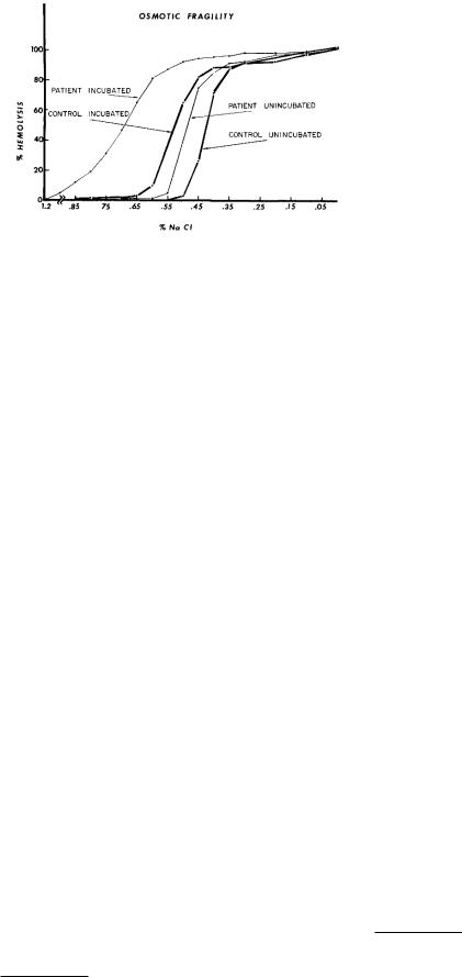
FIGURE 5.6. Osmotic fragility of red cells. The di erent curves are discussed in the text. From S. I. Rappoport (1971). Introduction to Hematology. New York, Harper & Row, p. 99. Reproduced by permission of Harper & Row.

mannitol are not reabsorbed at all. If they are present in the nephron, for example, from intravenous administration, the driving pressure of water is lowered and less water is reabsorbed than would be normally. The result is an increase in urine volume and a dehydration of the patient called osmotic diuresis.8 Similar diuretic action takes place in a diabetic patient who “spills” glucose into the urine.

5.4.6 Osmotic Fragility of Red Cells

Red cells (erythrocytes) are normally disk-shaped, with the center thinner than the rim. In the disease called hereditary spherocytosis the red cells are more rounded. If a red cell is placed in a solution that has a higher driving pressure than that inside the cell, water moves in and the cell swells until it bursts. Since cell membranes (as distinct from the lining of capillaries) are nearly impermeable to sodium, sodium is osmotically active for this purpose.

The osmotic fragility test consists of placing red cells in solutions with di erent sodium concentrations and determining what fraction of the cells burst. A typical plot of fraction vs. sodium concentration is shown in Fig. 5.6. Sodium concentration decreases and pd increases to the right along the axis.

The patient with hereditary spherocytosis has cells that will be destroyed at a lower external pd (higher sodium concentration) than normal, because the membrane is more permeable to the sodium.

If the red cells are incubated at body temperature in a sodium solution with the osmolality of plasma for 24 h, the fragility of hereditary spherocytosis cells is markedly increased. During this incubation period the concentration of sodium within the cell increases; the sodium can-

8Gennari and Kassirer (1974); Guyton (1991).

not escape rapidly when the external concentration is reduced, the driving pressure within the cell is lower than before incubation, and water flows into the cell even more rapidly.

5.5Volume Transport Through a Membrane

In this section and the next we develop phenomenological equations to describe the flow of fluid and the flow of solute through a membrane. These are linear approximations to the dependence of the flows on pressure and solute concentration di erences. Three parameters are introduced that are widely used in physiology: the filtration coe cient (or hydraulic permeability), the solute permeability, and the solute reflection coe cient.

The volume fluence rate or volume flow per unit area per second through a membrane is Jv .

(5.8) Consider pure water. The fluence rate depends on the pressure di erence across the membrane. When the pressure di erence is zero, there is no flow. The direction of flow, and therefore the sign of the fluence rate, depends on which side of the membrane has the higher pressure. The simplest relationship that has this property is a linear one:9

The proportionality constant is called the filtration coefficient or hydraulic permeability. It depends on the details of the membrane structure, such as the properties of the pores. The SI units for Lp are m s−1 Pa−1, m3 N−1 s−1, or m2 s kg−1. Often in the literature, however, values of Lp are reported in units of (cm/s)/atm. Since 1 atm = 1.01 × 105 Pa, the conversion is

1 cm s−1 atm−1 = 0.99 × 10−7 m s−1 Pa−1. (5.10)

If a solute is present to which the membrane is completely impermeable, only water will flow, and the flow will depend on ∆pd:

∆pd = pd − pd = p − π − (p − π )

=p − p − (π − π )

=∆p − ∆π

so

9The traditional sign convention has been followed here. There would be a minus sign in the equation if ∆p were defined to be p(x + ∆x) − p(x). However, it is usually defined as p − p . The flow is from the region of higher pressure to the region of lower pressure.

118 5. Transport Through Neutral Membranes

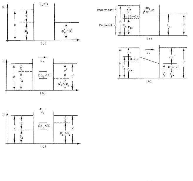
FIGURE 5.7. Di erent flow possibilities for a completely impermeant solute. (a) ∆pd = 0, so there is no flow even though p > p . (b) Flow to the right even though p = p . (c) Flow to the left even though p = p .

Figure 5.7 shows the pressure relations on each side of the membrane for no flow and for flow in either direction.

When the solute is partially permeant, the volume fluence rate in the linear approximation still depends on both ∆p and ∆π, but the proportionality constants may be di erent. Since the solute does not reduce the flow as much as in Eq. 5.11, it is customary to write the two constants as Lp and σLp:

Parameter Lp is determined by measuring Jv and ∆p when ∆π = 0, while σ is determined from measurements of ∆p and ∆π when Jv = 0.

Parameter σ is called the reflection coe cient. It has di erent values for di erent solutes. When σ = 0 there is no reflection, and the solute particles pass through like water. When σ = 1 all the solute particles are reflected and Eq. 5.12 is the same as Eq. 5.11.

FIGURE 5.8. Pressure relationships on each side of the membrane when σ = 23 . (a) There is no bulk flow. (b) There is flow to the right.

We can imagine that part of the solute moves freely with the water and part is reflected. (Later, we will consider a model for partial reflection in which a solute particle of radius a < Rp can enter the pore, but its center cannot be closer to the wall than its radius.) We can write

and we can further break this down to a driving pressure for the water pdw and one for the permeant solute:

osmotic pressure

of all solute molecules

Figure 5.8 shows the pressure relationships across the membrane.

In the approximation that van’t Ho ’s law holds, π =

In Eq. 5.16 the concentration is in molecules m−3; in Eq. 5.17 it is mol m−3. In both cases the units of kB T ∆C and RT ∆c are pascals.

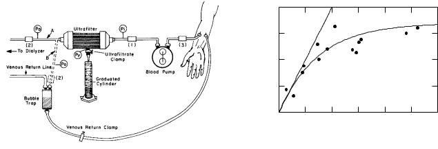
FIGURE 5.9. Apparatus used to treat fluid overload by ultrafiltration. Connection A is used for a patient connected to an artificial kidney. Connection B is used when the ultrafilter is used by itself. Pressure is monitored at Pi on the input side and Po on the output side. The three numbered rectangles are (1) the anticoagulant infusion site, (2) the site for measuring clotting time in the filter, and (3) the site for measuring patient clotting time. From M. E. Silverstein, C. A. Ford, M. J. Lysaght, and L. W. Henderson. Treatment of severe fluid overload by ultrafiltration. Reproduced, by permission, from the N. Engl. J. Med. 291: 747–751. Copyright c 1974 Massachusetts Medical Society. All rights reserved. Drawing courtesy of Prof. Henderson.

As an example of volume flow, consider ultrafiltration. Ultrafiltration is the process whereby water and small molecules are forced through a membrane by a hydrostatic pressure di erence while larger constituents are left behind. An interesting clinical application of ultrafiltration has been proposed. A severely edematous patient (for any of the reasons mentioned in the previous section) must have the extra water removed from the body. This is usually accomplished with diuretics, drugs that increase the renal excretion of water. Some patients may not respond to these drugs, and in other cases, particularly pulmonary edema, the response may not be fast enough. In the latter case, phlebotomy (bloodletting) is sometimes used to reduce the body water rapidly. This has obvious disadvantages, for example, the removal of blood cells. Silverstein et al. (1974) have used ultrafiltration to remove water and sodium from the plasma while leaving the other constituents behind. The apparatus is shown in Fig. 5.9. The ultrafilter consists of a total area S = 0.2 m2 of membrane, the permeability of which is 1 ml min−1 m−2 torr−1. The pores are permeable to molecules of molecular weight less than 50,000. The filtration rate is set by clamping the ultrafiltrate line (PF in Fig. 5.9), thereby increasing the pressure on the outside of the ultrafilter and decreasing the pressure drop across the membrane. The pressure was adjusted to give iv of 32 ml min−1 or less, which is equal to that found in a normal kidney.

FIGURE 5.10. Filtration rate (flow) iv , vs transmembrane pressure for a fixed blood flow of 200 ml min−1 through the apparatus in Fig. 5.9. The solid straight line shows a value of Lp of 1 ml min−1 m−2 torr−1 as reported by Silverstein et al. Modified, by permission, from the N. Engl. J. Med. 291: 747–751. Copyright c 1974 Massachusetts Medical Society. All rights reserved.

Figure 5.10 shows the flow vs ∆p. The initial slope of this curve determines LpS and hence Lp. The curve is not linear but saturates at about 32 ml min−1 of filtration flow, possibly because of poor mixing within the blood.

Ultrafiltration is sometimes called reverse osmosis. The name is unfortunate, because it suggests some mysterious process unrelated to the principles of this section. Ultrafiltration is often used by campers for purifying water and has been suggested for desalinization of sea water.

5.6Solute Transport Through a Membrane

Solute can pass through the membrane in two ways: it can be carried along with flowing water (solvent drag), and it can di use.

If there is no reflection (σ = 0) and the solute concentration is the same on both sides of the membrane so there is no di usion, the flux density or fluence rate is caused by solvent drag and is simply the solute concentration (particles per unit volume) times the volume fluence rate (Sec. 4.2):

Js = CsJv .

If the solute particles are completely reflected (σ = 1) then Js = 0.

In the intermediate case with coe cient σ,

Js = (1 − σ)CsJv .

This is consistent with the idea expressed by Eq. 5.14 that a fraction (1 − σ) of the solute particles can enter the membrane. In that case, Cs is the solute concentration outside the membrane on both sides, and Cs(1−σ) is

120 5. Transport Through Neutral Membranes

the solute concentration inside the membrane. We will develop a detailed model for transport in a right-cylindrical pore in Sec. 5.9. We anticipate that discussion and present a simple justification of the factor 1 − σ. In bulk solution the concentration Cs is obtained by imagining a certain volume of solution, counting the number of solute particles whose centers lie within the volume, and taking the ratio. In a cylindrical pore of radius Rp and length ∆Z, the volume of fluid is πRp2∆Z. The centers of solute particles of radius a cannot be within distance a of the pore wall. The number of solute particles within the pore is therefore Csπ (Rp − a)2 ∆Z. The concentration in the pore is the number of particles divided by the pore volume:

This correction is called the steric factor. Solvent flow within a distance a of the walls contributes to Jv but not to solvent drag. This model will be extended to a volume flow with a parabolic velocity profile in Sec. 5.9.4.

If Jv = 0 there will be no solvent drag but there will be di usion. The solute flux will be proportional to the concentration gradient and therefore to the concentration di erence across the membrane: Js ∆Cs. The proportionality constant depends on properties of the membrane. If the membrane is pierced by pores, for example, it depends on pore size, membrane thickness, number of pores per unit area, and the di usion constant. The dependence will be derived later in this chapter. It is customary to write the proportionality constant as ωRT : Js = ωRT ∆Cs. The factor ω is called the membrane permeability or solute permeability.

In the linear approximation the fluence rate resulting from both processes is the sum of these two terms:

Here an average value Cs has been written for the solvent drag term, because the concentration on each side of the membrane is not necessarily the same. The way that this average is taken will become clearer in the discussion of the pore model described in Section 5.9.

The solute equation has been written for both fluence rate and concentration in terms of particles. In terms of molar fluence rate and concentration, it is exactly the same:

Either way, the di usion proportionality constant is ωRT . It does not change because Cs and Js(particles) are both written in terms of particles, and cs and Js(molar) are both written in terms of moles. Referring to Eq. 5.18, the solvent drag term has units of (particles m−3) (m

s−1) = particles m−2 s−1. Therefore the factor ωRT has units of m s−1. Since the units of RT are joules or N m (per mole), the units of ω are

Further interpretation of ω will be made for specific models.

We have used the same σ in both the solvent drag term and in the preceding section. Although this was made plausible by saying that 1 − σ is the fraction of solute molecules that gets through the membrane, its rigorous proof is more subtle. It has been proved in general using thermodynamic arguments, which can be found in Katchalsky and Curran (1965). It can be proved in detail for specific membrane models.

5.7 Example: The Artificial Kidney

The artificial kidney provides an example of the use of the transport equations to solve an engineering problem. The problem has been extensively considered by chemical engineers, and we will give only a simple description here. Those interested in pursuing the problem further can begin with reviews by Galletti et al. (2000) or Lysaght and Moran (2000). The reader should also be aware that this “high-technology” solution to the problem of chronic renal disease is not an entirely satisfactory one. It is expensive and uncomfortable and leads to degenerative changes in the skeleton and severe atherosclerosis [Lindner et al. (1974)].

The alternative treatment, a transplant, has its own problems, related primarily to the immunosuppressive therapy. Anyone who is going to be involved in biomedical engineering or in the treatment of patients with chronic disease should read the account by Calland (1972), a physician with chronic renal failure who had both chronic dialysis and several transplants. The distinction between a high-technology treatment and a real conquest of a disease has been underscored by Thomas (1974, pp. 31–36).

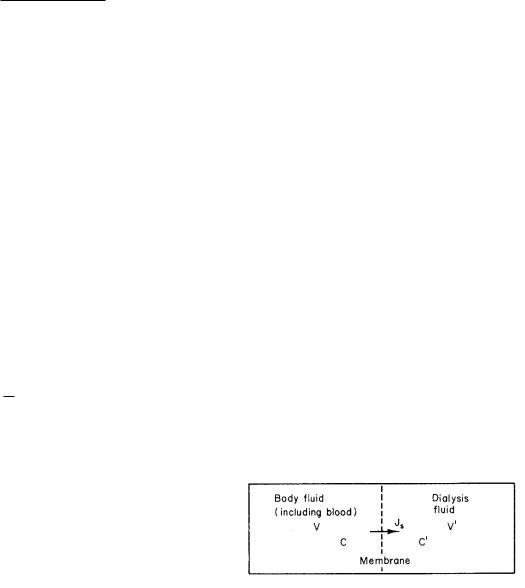
The simplest model of dialysis is shown in Fig. 5.11. Two compartments, the body fluid and the dialysis fluid, are separated by a membrane that is porous to the

FIGURE 5.11. The simplest model of dialysis. All the body fluid is treated as one compartment; transport across the membrane is assumed to take longer than transport from various body compartments to the blood.

small molecules to be removed and impermeable to larger molecules. If such a configuration is maintained long enough, then the concentration of any solute that can pass through the membrane will become the same on both sides. The dialysis fluid is prepared with the desired composition of such small molecules as sodium, potassium, and glucose. Volume V must be larger than V for e ective dialysis to take place; otherwise, the concentration of solutes in the dialysis fluid builds up from the initially prepared values. In early work, V was up to 100 l (since V is about 40 l). Although the fluid was replaced every 2 hours or so, it was an excellent medium in which to grow bacteria. Although the bacteria could not get through the membrane, they released exotoxins (or, if they died, endotoxins) which di used back into the patient and caused fever. Now a continuous flow system has been used in which the solutes are continually metered into flowing dialysis fluid that is then discarded. Because of this, we will assume that there is no buildup of concentration in the dialysis fluid. (E ectively volume V is infinite.) We will assume that ∆p = 0. (Actually, proteins cause some osmotic pressure di erence, which we will ignore.)

Without solvent drag, the solute transport is by di u- sion, Js = ωRT (C − C ), where C is the concentration of solute in the blood and C is the concentration in the dialysis fluid. If the surface area of the membrane is S, then the rate of change of the number of solute molecules

N is

dNdt = −SωRT (C − C ).

If the solute is well mixed in the body fluid compartment, then N = CV , and this equation can be written as

dCdt = −SωRTV (C − C ).

This is the equation for exponential decay. The steadystate solution is C = C . The complete solution is (Appendix F)

where the time constant is

The only variables that are adjustable in this equation are the membrane area S and its permeability ω. The size of pores in the membrane is dictated by what solutes are to be retained in the blood. The number of pores per unit area and the thickness of the membrane can be controlled. Typical cellophane membranes have ωRT = 5 × 10−6 m s−1 (with a thickness of 500 µm). The area may be 2 m2. With a fluid volume V = 40 l, this gives a time constant

have smaller permeabilities and therefore longer time constants, and rapid dialysis causes cerebral edema and severe headaches.

The actual apparatus is quite complicated. First, it must be sterile, which requires a sterilized, disposable dialysis membrane. Second, the apparatus causes clots, so the blood must be treated with heparin as it enters the machine, and the heparin must be neutralized with protamine as it returns to the patient.

5.8 Countercurrent Transport

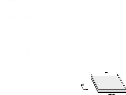
This section considers a problem that demonstrates the principle of countercurrent transport. An apparatus (perhaps a dialysis machine or an oxygenator) transports a single solute across a thin membrane of permeability ωRT . On one side of the membrane (the “inside”) is a thin layer of solvent that flows along the membrane in the +x direction as shown in Fig. 5.12. On the “outside” is another thin layer of solvent that may be at rest or may flow in either the +x or the −x direction. When it flows in the opposite direction of the fluid inside we have the countercurrent situation.

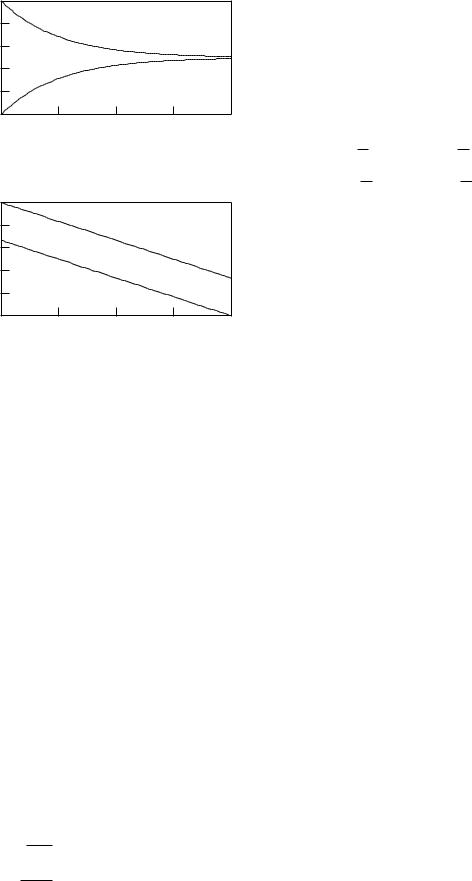
Suppose that the concentration of solute in the two layers is Cin(x) inside and Cout(x) outside. Solute is transported in the x direction in each fluid layer by pure solvent drag. It di uses through the membrane from the side with higher concentration to the other. We develop the model below and show that the steady-state concentration profiles are quite di erent depending on whether the solvent flows are in the same or opposite directions. The results are shown in Fig. 5.13 for the situation in which the value of Cin is 1 and the value of Cout is 0 where each solvent starts to flow across the membrane. In Fig. 5.13(a) both layers flow to the right; in Fig. 5.13(b) they flow in opposite directions. The countercurrent case is more effective in reducing Cin. The final value of Cin is 0.5 in the first case and 0.33 in the second.

To develop the model, we make the following assumptions. The concentration of solute in each fluid layer is independent of y, z, and t. The thickness of the fluid layer inside is hin. The fluid velocity jv in is everywhere constant. The only important mechanism for solute transport within the fluid is solvent drag. Let the length of

122 5. Transport Through Neutral Membranes

x

(b) The flows are in opposite directions.

FIGURE 5.13. Solute concentration profiles for two di erent situations where solvent flows parallel to the membrane surface and solute moves through the membrane from inside to outside. (a) Both fluid layers flow to the right. The concentrations rise and falls exponentially, eventually becoming the same on both sides of the membrane. (b) The countercurrent case, in which the solvent flows are in opposite directions. The solvent outside flows from right to left. The concentrations vary linearly.

the slab in the y direction be Y . Inside, the number of particles per second in through the face of the rectangle of area Y hin at x is Cin(x)jv inY hin. The number out through the face at x + dx is Cin(x + dx)jv inY hin. The number through the membrane into the exterior volume is [Cin(x) − Cout(x)] ωRT Y dx. Combining these we get

We restrict ourselves to the case in which |ain| = |aout| = a. Changing the direction of jv changes the sign of a. Assume a is the same on both sides. The equations show that the slope of Cin(x) is minus the slope of Cout(x) if both currents are in the same direction, and the two slopes are the same if the currents are in opposite directions. This can be seen in the solutions in Fig. 5.13.

You can verify that Eqs. 5.26 represent a solution of Eqs. 5.25:

Cin(x) = c21 1 + e−2ax + c22 1 − e−2ax ,

(5.26)

Cout(x) = c21 1 − e−2ax + c22 1 + e−2ax ,

were c1 and c2 are the values of Cin and Cout at x = 0. Figure 5.13(a) shows the concentrations for c1 = 1 and c2 = 0 with a = 1 and 0 < x < 2. If the sign of a is changed in the second di erential equation, then the fluid outside is flowing in the opposite direction to the fluid inside. Again you can verify that the most general solution is

Figure 5.13(b) is a plot with the constants set so that the concentration inside on the left is 1 and on the outside on the right is zero (c1 = 1, c2 = 2/3, a = 1, 0 < x < 2). This configuration is called countercurrent flow. We can see from the figure that the transport through the membrane is increased because the concentration di erence across the membrane is, on average, greater.

The countercurrent principle is found in the renal tubules [Guyton (1991), p. 309; Patton et al. (1989), p. 1081], in the villi of the small intestine [Patton et al. (1989), p. 915], and in the lamellae of fish gills [SchmidtNielsen (1972), p. 45]. The principle is also used to conserve heat in the extremities—such as a person’s arms and legs, whale flippers, or the leg of a duck. If a vein returning from an extremity runs closely parallel to the artery feeding the extremity, the blood in the artery will be cooled and the blood in the vein warmed. As a result, the temperature of the extremity will be lower and the heat loss to the surroundings will be reduced.

A similar expression can be derived for the exterior:

Our notation allows jv to have a di erent direction (sign). Defining a = ωRT /jv h we have the coupled di erential equations

dCin = −ain(Cin − Cout),

dx

(5.25)

dCout = +aout(Cin − Cout).

dx

5.9A Continuum Model for Volume and Solute Transport in a Pore

In this section we develop a model to predict the values of the phenomenological coe cients of Secs. 5.5 and 5.6. The success of the model depends on its ability to predict behavior, particularly as the size of solute particles is varied. This was an important problem in physiology in the 1960s and 1970s. Instead of comparing the model to experiment, we conclude the section by showing what the forces are on the membrane. This is important because

TABLE 5.1. Symbols used for porous membrane.

meant part of osmotic pressure plus water driving pressure

there has been a fair amount of confusion in the literature about the forces on a semipermeable membrane. This section is fairly long. It stands alone; you can skip it if you wish.

The model assumes that the membrane has a particularly simple structure.

1.The membrane is pierced by n circular pores per unit area, all having radius Rp and all being right cylinders. The membrane thickness is ∆Z.

2.The pore and the fluid are electrically neutral. No electrical forces are considered.

3.There is complete mixing on both sides of the pore, so that flow within the liquid on either side can be neglected.

4.The system is in the steady state. There is no variation in flux density (fluence rate) or concentration as a function of time.

5.The pores are large enough so that the bulk flow can be calculated by continuum hydrodynamics.

The quantities considered in this section are summarized in Table 5.1.

5.9.1 Volume Transport

The results of Chap. 1 can be used when the pore is filled with pure water or water and a solute for which σ = 0. From Eq. 1.40 the flux through a single pore is

The fluence rate through the membrane is obtained by multiplying iv by n, the number of pores per unit area.

While Lp can be measured fairly easily using Eq. 5.12, it is much more di cult to measure the microscopic quantities needed to test Eq. 5.29. We will not compare the model to experiment here;10 we will simply give an example of how calculations are done.

In discussing ultrafiltration we considered a filter (Fig. 5.10) for which Lp ≈ 1 ml min−1 m−2 torr−1. Since 760 torr = 1 × 105 Pa, the hydraulic permeability in SI units is

= 1.27 × 10−10 m s−1 Pa−1.

The manufacturer’s literature11 can be used to estimate

Rp ≈ 4.5 nm, ∆Z ≈ 10 µm.12

The viscosity of water is 0.9 × 10−3 Pa s at 25 ◦C. This gives us enough information to estimate n and the frac-

×(1.27 × 10−10 m s−1 Pa−1)

=7.1 × 1015 m−2.

Since the area of one pore is πRp2 = 6.36 × 10−17 m2, the total pore area in 1 m2 is 0.45 m2, a number that is not unreasonable.

Next consider the volume flow when the reflection co- e cient is not zero. The position within the pore is specified by cylindrical coordinates (r, φ, z). The position along the axis of the pore is given by z. The position in a plane perpendicular to the axis of the pore is specified by polar coordinates r and φ. Flow of the fluid is described by the vector volume fluence rate jv (r, φ, z). (We use J for fluence rate for the membrane as a whole and j for the fluence rate in bulk solution inside a pore.) It is possible to show rigorously that as long as the pore is a right circular cylinder, jv points only along z and is independent of φ (the fluid does not flow in a spiral and does not flow

The solution is in a steady state and the flow is not changing with time. Therefore, the flux density into a volume at z must be the same as the flux density out at z + dz:

10See earlier editions or, for example, Bean (1969, 1972).

11Amicon XM-50.

12This value nay not be consistent with the value of Lp quoted. The pore length ∆Z is not well known, and Lp is variable, depending on experimental conditions.

124 5. Transport Through Neutral Membranes

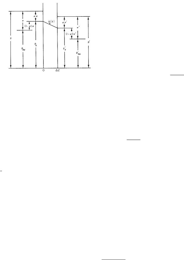
FIGURE 5.14. Pressure within a pore and at the boundaries in the steady state.

so that jv is constant along the z axis (although it can be a function of r). This is just what we saw in Chap. 1 for Poiseuille flow; the variation of jv with r corresponds to the parabolic velocity profile. A value of jv (r) that is constant in the z direction requires a constant value of ∂p/∂z inside the pore.

In the pore, the driving pressure is pd(z). A typical pressure profile is shown in Fig. 5.14. The symbols are defined in Table 5.1. The pressure in the pore has been drawn with constant slope, since ∂pd/∂z is constant. Us-

where Lp is given by Eq. 5.29. The value of σ is derived in the next section.

The average value of jv (r) within the pore will be called

jv . It is the total flux density through the pore divided by πRp2:

5.9.2 Solute Transport

We now consider solute transport in our model pore. The arguments here are very similar to those for combined di usion and solvent drag that were developed in Sec. 4.12. Those arguments are extended by averaging over the cross section of the pore.

Within the pore, the local solute flux is js(r, φ, z). Arguments similar to those in the preceding section can be o ered to show that js points along the z axis and is independent of φ:

The solute concentration does not depend on φ, or else there would be di usion in the φ direction and js would have a φ component. So C = C(r, z). The r dependence must be kept because the center of a solute molecule of radius a cannot be within a distance a of the wall. (Recall the discussion of the steric correction on p. 120.) Thus C(r, z) = 0 if r > Rp − a. We write13

The solute flux due to solvent drag is Csjv . For diffusion in one dimension the solute flux along the z axis is −D(∂C/∂z). For the cylindrical pore we can combine these and write

js(r, z) = C(r, z)jv (r, z) − D(r, a, Rp) ∂C(r, z) . (5.36) ∂z

The di usion constant has been written as a function of r, a, and Rp because in the pore, as distinct from an infinite medium, the constant depends on how close the particle is to the walls. (Remember the relation of D to the viscous drag and the fact that Stokes’ law requires modification when the fluid is confined in a tube.)

The preceding section showed that for the steady state jv is independent of z. A similar argument can be made using the continuity equation for solute particles, implying that js is independent of z. Therefore, Eq. 5.36 simplifies to

The easiest way to write C(r, z) in accordance with Eq. 5.35 is

C(r, z) = C(z)Γ(r),

This equation can be multiplied by 2πr dr and integrated from r = 0 to r = Rp. The result is

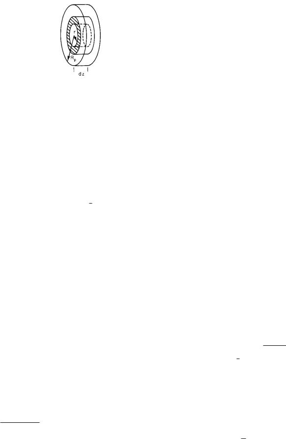
The physical meaning of this integration can be understood with the aid of Fig. 5.15, which shows a slab of fluid

13It can be argued that this is the only possible form for C(r, z). See Levitt (1975, p. 535 .).

FIGURE 5.15. A slab of fluid in a pore between z and z + dz, showing how the integration over r is done.

in the pore between z and z + dz. Solute does not cross a surface of constant r but moves parallel to the z axis. Di usion and solvent drag are considered in each shaded area 2πr dr. The integration of Eq. 5.38 establishes an average solute fluence rate, since the right-hand side of the equation is the total flux or current of solute particles per second passing through the pore:

Rp

is = js(r)2πr dr.

0

As with the volume fluence rate, it is convenient to call the average solute fluence rate js:

The first term of Eq. 5.38 is the di usive flux at z averaged over the entire cross section of the pore. Define an e ective di usion constant

The second term on the left of Eq. 5.38 is the solvent drag flux averaged over the entire cross section of the pore. The integral is

This integral can be evaluated because we know the velocity profile, jv (r), Eq. 1.39:14

We have already defined the average volume fluence rate

14This ignores the fact that since the walls a ect the force on the solute particles, the solute must distort the velocity profile slightly. This point is discussed below.

The desired quantity di ers only in the limits of integration. To calculate it, write

The integrals are easily evaluated (see Problems). The result is

This is a di erential equation for C(z). The right-hand side is the total solute fluence rate, which is constant. On the left-hand side, C varies along the pore so that the di usive and solvent-drag fluence rates add up to this constant value. If the constant in front of C(z) is written as

this is recognized as Eq. 4.58 for drift plus solvent drag in an infinite medium. The results of Sec. 4.13 can be applied here. It is only necessary to determine values for C0 and C0. Recall that in the pore C(r, z) = C(z)Γ(r). The function Γ(r) takes into account the reflection that occurs because solute particles cannot be closer to the pore wall than their radius. It was also assumed that the solution on either side of the membrane is well stirred. Therefore, C0 = Cs and C0 = Cs. Equation 4.70 becomes

This is an expression for js, the average solute fluence rate in the pore. To get solute fluence rate in the membrane,

Comparing this with the general phenomenological equation for solute flow, Eq. 5.18,

Js = (1 − σ)CsJv + ωRT ∆Cs