

Intermediate Physics for Medicine and Biology - Russell K. Hobbie & Bradley J. Roth
.pdf
|
|
|
8.2 The Magnetic Field of a Moving Charge or a Current |
207 |
||
|
P |
|
S |
S' |
|
|
|
|
|
|
|
|
|
r' |
|
r |
σ |
|
σ ' |
|
|
|
|
|
|
||
|
|
|
i |
E |
i |
|
i d s' |
|
|
i d s |
|
|
|
|
|
|
A |
b |
|
|
|
|
|
|
|
|
|
O
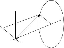
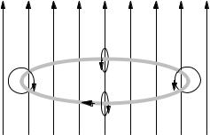
FIGURE 8.8. The magnetic field from a spherically symmetric radial distribution of current is zero. The source at O sends current uniformly in all directions. P is the observation point. For any element ds there is a corresponding ds such that ds×r = −ds ×r . The current through a small area dA around ds is i. The same current flows through a corresponding area around ds . Can you obtain the same result by a symmetry argument?
can be selected, such that ds × r = −ds × r . Associated with each element is a small area dA, and the current along ds is i = jdA. We can set dA = dA so i is the same in each case. Therefore, B = 0. (This can also be shown using Ampere’s law; see Problem 10.)
8.2.4 The Displacement Current
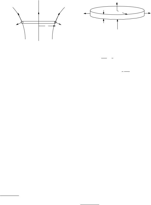
Derivation of Ampere’s law requires that there be no charge buildup, so that the total current through a closed surface is zero. However, we will consider an action potential in which the membrane capacitance charges and discharges. To see how this a ects Ampere’s law, consider current i charging the two shaded capacitor plates in Fig. 8.9. The area of each capacitor plate is A. The region between the plates, of thickness b, is filled with dielectric of
dielectric constant κ. The integral j · dS is i for surface S and zero for surface S . Because of the current, the charge density σ on the left-hand plate is increasing at a rate given by i = Adσ/dt, while on the right-hand plate the charge is decreasing because i = −Adσ/dt. Since the electric field between the plates is E = σ/κ 0 we can say that i = Ad(κ 0E)/dt. The quantity D = κ 0E is called the electric displacement, and
∂D jd = ∂t
is called the displacement current density. More careful consideration shows that Ampere’s law is valid when
FIGURE 8.9. A wire and capacitor plates are shown. The integral of the current density through surface S, which is pierced by the wire, is i. Through surface S , which is between the capacitor plates, the integral is zero. If the displacement current density is included, both surface integrals are the same. (If surfaces S and S are not large enough, there is also a net displacement current through S, as can be seen from Fig. 8.10.)
FIGURE 8.10. The conduction current (white arrows) and displacement current (black arrows) in a discharging capacitor are shown. The conduction current decreases with distance out the capacitor plates. The displacement current includes the fringing field. [From E. M. Purcell. Electricity and Magnetism, 2nd ed. Berkeley Physics Series, Vol. 2. New York, McGraw-Hill, 1985. Used by permission.]
there is charge buildup if we replace j by j + jd:
/ |
|
|
B · ds = µ0 |
(j + jd) · dS. |
(8.11) |
With this change, if S and S are circles of radius a, Ampere’s law gives B = µ0i/2πa for either one. (The radius of the circle must be very large; see the discussion in the next paragraph.)
What current should be used in the Biot–Savart law? A very surprising answer is that as long as the fields are relatively slowly varying (so that the emission of radio waves is not important), the displacement current contributes nothing. We are free to include it or ignore it. Purcell (1985, p. 328) and Shadowitz (1975, p. 416) discuss why this is so. It is not always easy to calculate the entire displacement current. For example, Fig. 8.10 shows how the conduction current and displacement current vary when
208 8. Biomagnetism
current charges a capacitor. Notice that some of the displacement current flows to and from the back sides of the capacitor plates. This is why we said in the previous paragraph that the radius of the curve defining surfaces S and S must be very large in order that one surface have no net flux of displacement current and the other have all of it. Whatever their size, however, Eq. 8.11 is valid.
It was mentioned above that a steady current from a point source that spreads uniformly in all directions generates no magnetic field according to the Biot–Savart law. Yet any circular loop has current flowing through it, so Ampere’s law suggests that there is a field. The discrepancy is resolved by noting that the current comes from a charge q at the origin that is being drained o by i = −dq/dt. This gives rise to a displacement current jd that cancels j (see Problem 10).
8.3The Magnetic Field Around an Axon
We can use the Biot–Savart law to calculate the magnetic field due to an action potential propagating down an infinitely long axon stretched along the x axis and embedded in an infinite homogeneous conducting medium. Section 7.1 showed that there are three components to the current: ii along the interior of the axon, dio out through the membrane (including both displacement current and conduction current), and current in the surrounding medium.
The principle of superposition allows us to calculate the field due to the exterior current by finding the magnetic field dB from current dio into the surrounding medium from axon element dx, and then integrating along the axon.
We saw in Chapter 7 that the current in the external medium from a small element dx flows uniformly in all directions from a point source. We learned in the preceding section that the magnetic field generated by a spherically symmetric radial current is zero. Therefore, in the approximation that the axon is very thin, we can ignore the external current from each element dx. We can do this only because the medium is infinite, homogeneous, and isotropic. When the exterior conductor has boundaries or structure, the symmetry is broken and the external currents contribute to the magnetic field. Our calculation breaks down very close to the axon. Distortions from the field due to the external current because the axon is not infinitely thin are about 1% close to the axon. The current through the cell membrane gives a very small contribution to the magnetic field—roughly 1 part in 106.
The major contribution is therefore from ii. We use the law of Biot–Savart, Eq. 8.10. The observation point is in the xy plane at (x0, y0, 0) and the axon lies along the x axis so that ds = x1 dx, as shown in Fig. 8.11. The
B 
|
z |
(x 0,y0 |
,0) |
|
|
||
y |
|
r |
x |
|
|
|
|
|
|
θ |
Line |
|
|
px |
|
|
|
of B |
FIGURE 8.11. The geometry for calculation of the magnetic field due to a current element i dx or current dipole px stretched along the x axis.
product ds × r can be evaluated using Eq. 1.8 or 1.9:
|
|
|
|
x |
y |
z |
|
|
|
|
|
|
|
|
|
1 |
1 |
1 |
|
|
|
|
|
ds r = |
|
|
dx |
0 |
0 |
|
= dx y |
0 |
z. |
||
× |
|
|
|
|
|
|
0 |
|
|
1 |
|
|
x |
0 |
− |
x y |
0 |
|
|
|
|||
|
|
|
|
|
|
|
|
|
|||
The term in the denominator is r3 = (x0 − x)2 + y02 3/2. The magnetic field in the xy plane is in the z direction and has magnitude
Bz = |
µ0y0 |
|
ii(x) dx |
. |
|
[(x0 − x)2 + y02]3/2 |
|||
|
4π |
|
||
It was shown in Eq. 7.17 that ii = −πa2σi(dvi/dx). The final expression for Bz is
Bz = − |
µ0a2σiy0 |
|
|
[dvi(x)/dx] dx |
(8.12) |
|
|
|
|
|
. |
||
4 |
|
[(x0 − x)2 + y02]3/2 |
||||
The computer program in Fig. 8.12 evaluates the field for the same crayfish axon whose external potential was studied in Sec. 7.4. The field at a distance 2a from the axon is plotted in Fig. 8.13. Again, the results agree well with more sophisticated calculations [Swinney and Wikswo (1980); Woosley et al. (1985)]. The latter reference is particularly clear and should be accessible to those who have studied the convolution integral in Chapter 12. A three-dimensional plot of their results is shown in Fig. 8.14.
It is worth repeating that a calculation this simple succeeds only because the axon and the exterior medium are infinite. If there are boundaries, or if there are regions in the external medium where the conductivity changes, then current in the external medium does contribute to the magnetic field. For example, an isolated nerve preparation in air would have the external current flowing in a thin layer of ionic solution along the outside of the axon, where it would generate a field that almost completely cancels that from ii.
An approximation valid at large distances can be obtained from Eq. 8.12 by expanding the denominator in

8.4 The Magnetocardiogram |
209 |
1.0 |
|
|
|
|
0.5 |
|
|
|
|
0.0 |
|
|
|
|
B, nT |
|
|
|
|
-0.5 |
|
|
|
|
-1.0 |
|
|
|
|
-1.5 |
5 |
10 |
15 |
20 |
0 |
||||
|
|
x0, mm |
|
|
FIGURE 8.13. The magnetic field Bz 0.12 mm from a crayfish axon in an infinite homogeneous conducting medium is shown. The field was calculated using the program of Fig. 8.12. The exterior potential for this configuration was calculated in Sec. 7.4.
FIGURE 8.12. The program used to calculate the magnetic field outside an axon in an infinite homogeneous conductor using Eq. 8.12. It uses the Romberg integration routine qromb from Press et al. (1992).
much the same way we did to obtain Eqs. 7.26 and 7.27. The observation point is (R, θ) in the xy plane. In this case we need the expansion of
1 |
|
1 |
|
|
|
|
x |
|
|
x2 −3/2 |
||
|
= |
|
|
1 − |
2 |
|
cos θ + |
|
|
|
||
r3 |
R3 |
|
R |
|
R2 |
|||||||
|
|
1 |
|
1 + |
3x cos θ |
+ |
|
|||||
|
≈ |
|
|
|
|
|
· · · . |
|||||
|
R3 |
|
|
|
R |
|||||||
The final result is
Bz = µ0 πa2 σi sin θ (vi(x1) − vi(x2))
+ |
µ0 πa2 |
σi3 sin θ cos θ |
x2 |
|
x2 |
|
|
|
xvi(x)|x1 |
+ |
|
vi(x) dx . |
|
|
4πR3 |
x1 |
||||
|
|
|
|
|
|
(8.13) |
The first term is proportional to the current dipole, p defined for the depolarization in the previous chapter. For a complete pulse the first term vanishes and the second term is used.
FIGURE 8.14. A three-dimensional plot of the magnetic field around the crayfish axon. The minimum distance from the axon is 0.5 mm.
8.4 The Magnetocardiogram
It is now feasible to measure magnetic fields arising from the electrical activity of the heart (the magnetocardiogram or MCG) and the brain (the magnetoencephalogram or MEG). The models developed in Sec. 8.3 and in Chapter 7 can be used to compare the electric and magnetic signals from a current dipole p. The instrumentation for these measurements is described in Sec. 8.9.
For a single cell at the origin in a homogeneous conducting medium, the exterior potential at observation
210 8. Biomagnetism
point r is given by Eq. 7.13:
p · r
v = 4πσor3 .
The current dipole p points along the cell in the direction of the advancing depolarization wave and has magnitude [Eq. 7.12] p = πa2σi∆vi. An expression analogous to Eq. 7.13 describes the magnetic field of a depolarizing cell. We consider the field due to current along the x axis and then generalize the result. The derivation begins with Eq. 8.13 and uses the geometry of Fig. 8.11. The region of depolarization occupies only a millimeter or so along the cell. Since the measurements are made much farther away, the denominator can be removed from the integral, which
is then just (dv/dx) dx. If the depolarization is at the origin, then the expression for Bz for z = 0 is
B |
z |
= |
− |
µ0a2σiy0 [v(x2) − v(x1)] |
= |
µ0 py0 |
. |
||
|
|
4(x02 + y02)3/2 |
|
4π |
|
(x02 + y02)3/2 |
|
||
(8.14) Figure 8.11 shows that y0 = r sin θ, so that py0 = p r sin θ = |p × r|. The direction of B is also consistent with the cross product. Generalizing, we have for a single cell,
p × r
B = µ0 4πr3 . (8.15) Note the remarkable similarity between Eqs. 7.13 and 8.15. One involves the dot product, and the other the cross product. For both, the field falls as 1/r2. If we are considering the cardiogram, either field from the entire heart is the superposition of the field from many cells. As with the electrocardiogram, the first approximation for the magnetocardiogram is to ignore changes in 1/r2 and speak of the total current-dipole vector.
Measurements of either the potential or the magnetic field can be used to determine the location of p. We will adopt the coordinate system usually used for the magnetocardiogram. The x axis points to the patient’s left, the y axis points up, and the z axis points toward the front of the patient, roughly perpendicular to the chest wall. Assume that p is at the origin and the anterior chest surface is the xy plane at some fixed value of z. We ignore distortions to the field which arise because no current can flow in the region beyond the body, and we assume that the conductivity of the body is homogeneous and isotropic. From Eq. 8.15, we obtain the three components of B along the line (x, 0, z):
Bx = |
µ0py z |
, |
|
|
|
||
|
|
|
|
||||
|
|
|
4πr3 |
|
|
||
By = |
µ0 (pz x − zpx) |
, |
(8.16) |
||||
|
|
|
4πr3 |
|
|
||
Bz = − |
µ0py x |
|
|
||||
|
. |
|
|
||||
4πr3 |
|
|
|||||
Compare these results to the lines of B in Fig. 8.15, which were drawn for the three components of p using the right-hand rule. Along the line being considered
y
x
px
(a)
y
x
py
(b)
y
x
pz
(c)
(x 2 , 0,
0, z)
z)
(x1, 0,
0, z )
z )
z
(x 2 , 0, z)
0, z)
(x1, 0,
0, z )
z )
z
(x 2 , 0,
0, z)
z)
(x1, 0,
0,
 z )
z )
z
FIGURE 8.15. The magnetic field produced by the three components of a current dipole at the origin. The coordinate system is that customarily used for magnetocardiography. The x axis points toward the subject’s left, the y axis is vertical, and the z axis points forward through the subject’s chest. The coordinate system is viewed over the subject’s right shoulder.
(y = 0, z = const), px contributes only to By , and By is always negative. Component py contributes to both Bx and Bz ; the latter changes sign while the former does not, as we change the value of x. Component pz gives only a y component of B that changes sign as x changes sign. The component normal to the body surface, Bz is given
by |
µ0 py x |
||||
Bz (x, 0, z) = − |
|||||
|
|
|
. |
||
4π |
(x2 + z2)3/2 |
||||
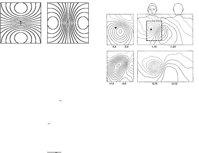
Figure 8.16 plots contours for the potential and the magnetic field component Bz perpendicular to the body surface when p points along the y axis. Again, distortions because of changes in conductivity are ignored. The similarity of the two sets of contours is clear. The contours of constant potential are proportional to py y/r3, while the contours for Bz are proportional to −py x/r3. Either
8.5 The Magnetoencephalogram |
211 |
+ |
y |
− |
x |
(a) Potential, v
y |
+ |
− |
|
|
x |
(b) Magnetic field, Bz
FIGURE 8.16. Contour plots in the xy plane for (a) the potential and (b) the z component of the magnetic field from a current dipole p pointing along the y axis, calculated for an infinite, isotropic conducting medium.
contour map can be used to determine the location and depth of p. To be specific, consider the contours for Bz . The field is proportional to the function x/(x2 + z2)3/2,
which changes sign right over the source and has a max-
√
imum and a minimum at x = ±z/ 2. The depth of the source z is related to the spacing ∆x along the x axis between the maximum and minimum by
∆x |
|
z = √2 . |
(8.17) |
The source is located directly beneath the point on the axis where Bz = 0, and its strength is related to the maximum value of Bz by
µ0py
Bz (max) = √ . (8.18) 6π 3z2
Figure 8.17 shows real maps of the potential and the magnetic field on the surface of the chest. While the basic features are described by the simple current dipole model, the exact shape of the contours in Fig. 8.17 di ers from the shape in Fig. 8.16. This is due to variations in conductivity of the body. The surface potential is distorted by conductivity di erences throughout the thorax; the magnetic field is particularly susceptible to return currents flowing just below the surface of the body. Hosaka et al. (1976) did an early calculation of the e ect of currents at the surface of the torso on the magnetocardiogram. They found that the return current modifies the component of B perpendicular to the body surface by about 30%. Tangential components of B are influenced more; this is why the normal component Bz is usually measured. Other calculations have been done by Purcell et al. (1988). Tan et al. (1992) show that using a model of the conductivities that matches the geometry of the patient’s thorax allows accurate localization of the current dipole source from the surface measurements. Stroink (1993) reviews magnetic field maps; surface potential maps are reviewed by Taccardi and Punske (2004) and by Stroink et al. (1996).
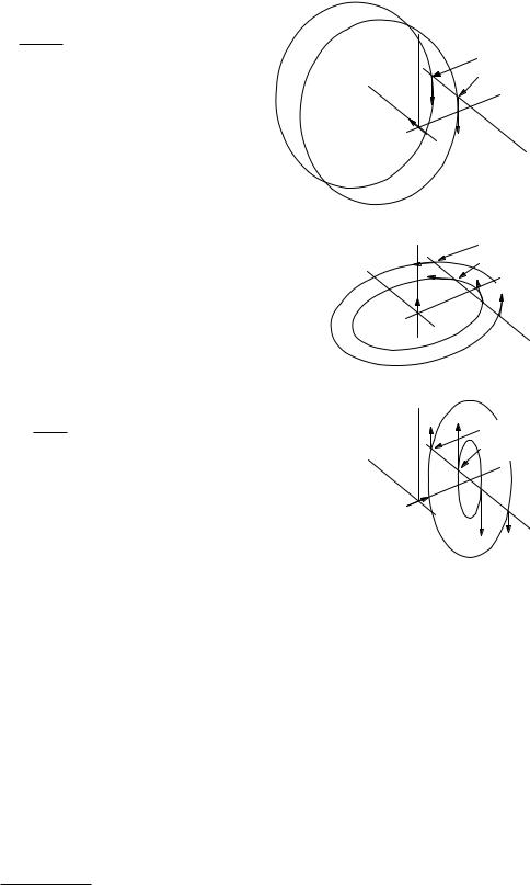
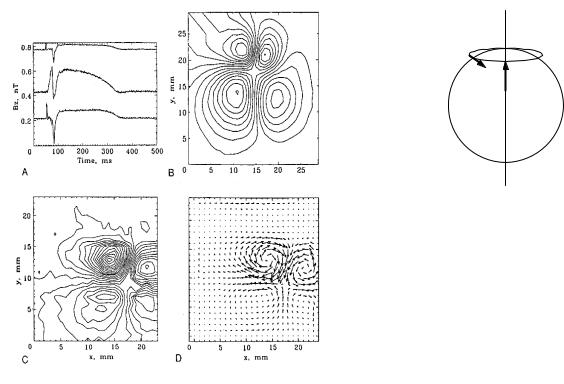
The magnetic field close to the heart is a ected by the anisotropy of the tissue conductivity. Figure 8.18 shows measurements made 1.5 mm from a 1-mm-thick
FIGURE 8.17. Maps of the magnetic field perpendicular to the body (left) and the body surface potential (right) in two patients. The upper row is for a normal patient, and the lower row for a patient with an anterior myocardial infarction. The dashed rectangle in the potential map corresponds to the area for which the magnetic field was measured. The dot in the upper row shows where the midline intersects the level of the fourth intercostal space. Note how the constant contours for the magnetic field are oriented at right angles to the isopotential lines, as in the previous figure. From G. Stroink, Cardiomagnetic Imaging. In R. A. Dunn and A. S. Berson, eds.
Frontiers in Cardiovascular Imaging. Raven Press, 1992. pp. 161–177. Used by permission.
slice of canine myocardium by Staton et al. (1993). Panel A shows the time course of simultaneous recordings from three pickup coils 3 mm in diameter and separated by 4 mm. There are striking di erences over 4 mm. Panel B shows a magnetic field contour map during stimulus from another experiment. Instead of having one peak and one valley as in Figs. 8.16 and 8.17, it shows a cloverleaf or quatrefoil pattern. Panels C and D show the field contours and the current flow in a third experiment, 6 ms after stimulation. This field and current pattern is predicted by bidomain calculations [Wikswo (1995b)].
8.5 The Magnetoencephalogram
The magnetic signals from a nerve action potential are weaker than those from the heart for two reasons. First, the current-dipole vector associated with the repolarization follows close behind the depolarization and reduces the field. (The largest unmyelinated axons in the body have a conduction speed of about 1 m s−1 and the pulse is about 1 mm long. Myelinated fibers have a pulse length up to 8–10 times longer.) Second, the cross-sectional area of the advancing wavefront is much smaller. However,
212 8. Biomagnetism
FIGURE 8.18. The results of magnetic field measurements very close to a slice of canine myocardium. The panels are described in the text. Part of the figure is reproduced from J. P. Wikswo, Jr. Tissue anisotropy, the cardiac bidomain, and the virtual cathode e ect. In D. P. Zipes and J. Jalife, eds. Cardiac Electrophysiology: From Cell to Bedside, 2nd ed. pp. 348–361, c 1995 Elsevier, Inc., with permission of Elsevier. The rest is from D. J. Staton, R. N. Friedman, and J. P. Wikswo, Jr. (1993). High-resolution SQUID imaging of octupolar currents in anisotropic cardiac tissue. IEEE Trans. Appl. Superconduct. 3(1):1934–1936. c 1993 IEEE.
the magnetic fields accompanying action potentials have been measured in nerve [Barach et al. (1985); Roth and Wikswo (1985)] and in muscle [Gielen et al. (1991)]. They have also been measured in green algae [Trontelj et al. (1994)].
We saw in Sec. 6.1 that nerve cells have an input end (dendrites), a cell body, and an axon. The signal that propagates from a synapse through the dendrites to the cell body and axon is much smaller (about 10 mV) and longer (10 ms) than an action potential that travels along the axon. The cells at the surface of the cerebral cortex have dendrites that are like the trunk of a tree perpendicular to the surface of the cortex, with branches from several directions coming to the trunk. The signal from the trunk is the primary contributor to the magnetoencephalogram (MEG)and electroencephalogram (EEG). The problems show that the magnetic field associated with the rise of the post-synaptic potential is more easily observed outside the brain than is the action potential.
B
p
FIGURE 8.19. A current dipole p is oriented radially inside a homogeneous conducting sphere. The return current is independent of the azimuthal angle, φ. By symmetry the magnetic field, if any, must be in the φ direction; the current in Ampere’s circuital law, which is the sum of the current in p and the return current, is zero.
One can see from the symmetry argument in the caption of Fig. 8.19 that in a spherically symmetric conducting medium the radial component of p and its return currents do not generate any magnetic field outside the sphere. Therefore the MEG is most sensitive to detecting activity in the fissures of the cortex, where the trunk of the post-synaptic dendrite is perpendicular to the surface of the fissure. A tangential component of p does produce a magnetic field outside a spherically symmetric conductor. The extracellular current does not contribute to the radial component of the magnetic field [H¨am¨al¨ainen et al. (1993)], so Eq. 8.15 gives Br correctly. Extracellular current does influence the tangential components of the magnetic field. Since the skull is not a perfect sphere, there is some e ect of the radial component of p on the MEG. The EEG is sensitive to both radial and tangential components of p. The information available from the EEG and MEG has been reviewed by Wikswo et al. (1993).
Measurements of the magnetoencephalogram are often based on evoked responses. A repetitive stimulus is presented to the subject—audible, visual, or tactile—or the subject is asked to perform a repetitive task such as flexing a finger. Signal-averaging techniques are used to identify the associated changes in magnetic field (see Chapter 11). Figure 8.20 shows averaged magnetic field contours measured over the scalp of a subject who heard a string of words presented in random order every 2.3 s. Sometimes the subject was asked to read something else and ignore the words. At other times the subject was asked to pay attention and count how many of the words were on a list. The first peak, 100 ms after presentation of the word, was the same in both cases. The sustained field peak, SF, was considerably stronger when the subject was paying attention to the list. Magnetic contours and the equivalent current dipole source are also shown.
Magnetic measurements have also been made of slower signals. Grimes et al. (1985) found ion currents in the

FIGURE 8.20. Magnetic field maps recorded over the scalp of a subject who heard a series of words and either ignored them by reading something else or listened carefully and counted how many of the words were in a predetermined list. The features are discussed in the text. Reprinted with permission from M. H¨am¨al¨ainen, R. Harri, R. J. Ilmoniemi, J. Knuutila and O. V. Lounasmaa. Magnetoencephalography—theory, instrumentation, and applications to noninvasive studies of the working human brain. Revs. Mod. Phys. 65(2): 413–497 1993. Copyright 1993 by the American Physical Society.
human leg that change over an hour or so. Thomas et al. (1993) found a quasistatic ionic current in the chick embryo, probably associated with active-transport pumps. Richards et al. (1995a) have measured a magnetic signal associated with slow currents in the small intestine of the rabbit and its supporting mesentery. The signal changes appreciably if the blood supply to the intestine is cut o . These measurements could be clinically useful, because mesenteric ischemia is di cult to diagnose early [Richards et al. (1995b), Petrie et al. (1996)].
8.6 Electromagnetic Induction
In 1831 Faraday discovered that a changing magnetic field causes an electric current to flow in a circuit. It does not matter whether the magnetic field is from a permanent magnet moving with respect to the circuit or from the changing current in another circuit. The results of many experiments can be summarized in the Faraday induction law :
/ |
E · ds = − |
d |
B · dS = − |
dΦ |
(8.19) |
||
|
|
|
|
. |
|||
|
dt |
dt |
|||||
8.6 Electromagnetic Induction |
213 |
It states that the line integral of E around a closed path is equal to the negative of the rate of change of the magnetic flux through any surface bounded by the path. The relationship between the direction of S and ds is given by a right-hand rule: if the fingers of the right hand curl around the circuit in the direction of ds, the thumb of the right hand points in the direction of a positive nor-
mal to S. The units of magnetic flux Φ = B ·dS are T m2 or weber (Wb). Rapidly changing magnetic fields can induce currents large enough to trigger nerve impulses. This is discussed in Sec. 8.7.
The di erential form of the Faraday induction law is (see Problem 20)
curl E = × E = − |
∂B |
(8.20) |
|
|
. |
||
∂t |
|||
The result of the vector operation curl is another vector. In Cartesian coordinates the components of × E are
( × E)x = |
∂Ez |
|
− |
∂Ey |
, |
∂y |
|
∂z |
|||
( × E)y = |
∂Ex |
|
− |
∂Ez |
, |
∂z |
|
∂x |
|||
( × E)z = |
∂Ey |
|
− |
∂Ex |
. |
∂x |
|
∂y |
These can be abbreviated by using determinant notation as
|
|
|
x |
|
y |
|
z |
|
|
|
|
|
1 |
|
1 |
1 |
|
|
|||
|
|
|
∂ |
|
∂ |
|
∂ |
|
(8.21) |
|
( |
E) = |
|
|
|
|
|
|
|
. |
|
∂x |
|
∂y |
∂z |
|||||||
× |
|
|
|
|
||||||
|
|
Ex |
Ey |
Ez |
|
|
||||
|
|
|
|
|||||||
Similarly (Problem 21) the di erential form of Ampere’s law is
|
|
∂D |
|
|
curl B = × B = µ0 |
j + |
|
. |
(8.22) |
∂t |
The integral form of the Faraday induction law can be used to determine E only if the symmetry is such that E is always parallel to ds and has the same magnitude all along the path. One situation where it can be used is a circular loop of wire in the xy plane centered at the origin. The radius of the loop is a and its normal is along the +z axis. Suppose that everywhere in the xy plane within the boundary of the circle the field points along z and depends only on time: B(x, y, z, t) = B(t)1z. Symmetry shows that E has the same magnitude everywhere in the wire and is always tangent to the loop. Equation 8.19 gives
E = − |
a dB |
(8.23) |
2 dt . |
If the loop is made of material that obeys Ohm’s law, there is a current of density j = σE = −(σa/2)(dB/dt). If the radius of the wire is b (b a), then i = −(σπab2/2)(dB/dt). Figure 8.21 shows the direction of the induced current if dB/dt is positive. The induced
214 8. Biomagnetism
i
FIGURE 8.21. A magnetic field increasing in the direction shown induces a current in the loop. This current generates a magnetic field in the opposite direction, opposing the change in the magnetic field.
current sets up its own magnetic field which points in the −z direction within the loop, opposing the primary field increase within the loop. The induced current always opposes the change of magnetic field that produces it. This is called Lenz’s law. If it were not true, the induced current, once started, would increase indefinitely.
This result does not require that the ring be hollow; it can be part of a much larger conductor. The larger the conductor, the greater the radius of the path along which the induced current can flow. The currents that changing magnetic fields induce in conductors are called eddy currents and cause heating losses in the conductor. Iron, which is a conductor, is often used as a core in transformer windings to increase the intensity of the magnetic field. To reduce the eddy-current losses, the cores are made of thin layers of iron insulated from one another by varnish. This limits the radius of the path in which the eddy currents can flow. Some coils and transformers are wound on cores of powdered iron dispersed in an insulating binder. Rooms with thick conducting walls (aluminum, about 2 cm thick) have been used to shield against 60 Hz magnetic fields from power wiring. The eddy currents induced in the aluminum attenuate the field by about a factor of 200 [Stroink et al. (1981)].
a |
· |
ds is the work done per unit charge |
The quantity b E |
|
in moving from a to b and is called the electromotive force along the path from a to b. Terminology is not always consistent; see the discussion by Page (1977). The details of how a changing magnetic field causes a current to flow were shown above for a circular conductor. The force on a moving charge due to the induced electric field is balanced by the drag force as the charge drifts through the conductor. Energy supplied by the changing magnetic field is dissipated as heat. If a voltmeter is attached to two points on the circle, the voltmeter reading may seem paradoxical, until one realizes that there may be changing flux in the voltmeter leads as well. An additional complication is that when there is any region of space in which
b
× E = 0, then it is possible for a E · ds to depend on the path (rather than just the end points), even if the
magnetic field is zero at all points on the path. This is described clearly and in detail by Romer (1982).
8.7 Magnetic Stimulation
Since a changing magnetic field generates an induced electric field, it is possible to stimulate nerve or muscle cells without using electrodes. The advantage is that for a given induced current deep within the brain, the currents in the scalp that are induced by the magnetic field are far less than the currents that would be required for electrical stimulation. Therefore transcranial magnetic stimulation (TMS) is relatively painless. Magnetic stimulation can be used to diagnose central nervous system diseases that slow the conduction velocity in motor nerves without changing the conduction velocity in sensory nerves [Hallett and Cohen (1989)]. It could be used to monitor motor nerves during spinal cord surgery, and to map motor brain function. Because TMS is noninvasive and nearly painless, it can be used to study learning and plasticity (changes in brain organization over time). Recently, researchers have suggested that repetitive TMS might be useful for treating depression and other mood disorders.
One of the earliest investigations was reported by Barker et al. (1985) who used a solenoid in which the magnetic field changed by 2 T in 110 µs to apply a stimulus to di erent points on a subject’s arm and skull. The stimulus made a subject’s finger twitch after the delay required for the nerve impulse to travel to the muscle. For a region of radius a = 10 mm in material of conductivity 1 S m−1, the induced current density for the field change in Barker’s solenoid was 90 A m−2. (This is for conducting material inside the solenoid; the field falls o outside the solenoid, so the induced current is less.) This current density is large compared to current densities in nerves (Chap. 6).
Magnetic stimulators are relatively high-power devices, requiring thousands of amps passed through coils for a few hundred microseconds. Most magnetic stimulators are capacitor discharge devices, in which a large capacitor is charged to a high voltage (several kV) and then discharged through the coil. Di erent coil geometries have been examined; the most common one is a figure-of-eight shape. Several theoretical analyses and models have been made, including those by Heller and van Hulsteyn (1992) and Esselle and Stuchly (1995). Magnetic stimulation is included in the review by Roth (1994) and is compared to other brain imaging methods by Ilmoniemi et al. (1999).
8.8Magnetic Materials and Biological Systems
Just as the electric field can be altered by the polarization of a dielectric, the magnetic field can be altered by
|
|
8.8 Magnetic Materials and Biological Systems |
215 |
|
z |
|
|
Bz(z +dz ) |
|
B |
|
B |
a |
|
m |
|
dz |
|
Br( a ) |
i |
|
|
||
|
i |
|
|
|
d F |
a |
d F |
Bz( z ) |
|
FIGURE 8.22. A current loop in an inhomogeneous magnetic field experiences a force toward the region of stronger magnetic field. The circular loop lies in a plane perpendicular to the z axis. Current flows into the page on the right and out of the page on the left.
matter. Biological measurements can be based on alterations of the field by an organ in the body. Some cells exhibit permanent magnetism, which is important for measuring direction in some bacteria, birds and other organisms.
8.8.1 Magnetic Materials
The e ects of magnetic fields on material are more complicated than those of electric fields. Since there are no known magnetic charges (monopoles), we must consider the e ect of magnetic fields on current loops or magnetic dipoles. Figure 8.22 shows a current loop in a magnetic field that decreases as z increases. As a result the lines of B spread apart. The loop has radius a, carries current i, and has magnetic moment1 m. For the orientation shown, there is a force on the loop in the −z direction that is toward the region where the field is stronger. If the magnetic moment of the loop were not parallel to B, there would also be a torque on the loop. For ease in calculation, imagine that the loop has been placed in the field in such a way that along the axis of the loop, B points in the z direction. Then the spreading of the lines of B means that B has a component radially outward all around the loop. Because of the symmetry Br has a constant magnitude everywhere around the loop, and the force on the loop is −2πa i Br (a).
Field Br (a) is found by considering the fact that the total magnetic flux through all surfaces of the pillbox in Fig. 8.23 is zero (Eq. 8.6). The net outward flux is
[Bz (z + dz) − Bz (z)] πa2 + Br (a)2πa dz = 0.
1Be careful. We are talking about two di erent kinds of dipoles in this chapter. The current dipole p is a source and sink of current and has units A m. The magnetic dipole m, equivalent to a small magnet with north and south poles, has units A m2. The magnetic field from a magnetic dipole falls o as 1/r3.
FIGURE 8.23. Gauss’s law for B is applied to a pillbox of radius a and thickness dz.
This can be rearranged to give
∂B∂zz + a2 Br (a) πa2 dz = 0,
from which
Br (a) = −a2 ∂B∂zz .
The force on the loop is therefore
Fz = πa2i |
∂Bz |
= mz |
∂Bz |
. |
(8.24) |
∂z |
|
||||
|
|
∂z |
|
||
If m is parallel to B the force is toward the region of stronger field; if m is antiparallel to B the force is toward the region of weaker field.
An atom can have a magnetic moment because of two e ects.2 The motion of the electrons in orbit about the nucleus constitutes a current, as a result of which there may be an orbital magnetic moment. The intrinsic spin of each electron gives rise to a spin magnetic moment, independent of any orbital motion. In most atoms, the orbital magnetic moments average to zero, and most of the electrons are arranged in pairs whose spins cancel. The atom therefore usually has no net magnetic moment.
Most substances placed in an inhomogeneous field experience a weak force away from the region of strong field, and the force is roughly proportional to the square of the field strength, an e ect called diamagnetism. It can be understood with a simple classical model. As the atom is moved into the magnetic field, the Faraday induction e ect distorts the orbits of the electrons to induce a magnetic dipole moment proportional to B and in the opposite direction, consistent with Lenz’s law. The force is therefore proportional to Bz (∂Bz /∂z). Purcell (1985) has a quantitative treatment of this model.
A few substances are attracted to the region of stronger field, again with a force that is often proportional to the square of the field. Each atom of these paramagnetic substances has a permanent magnetic moment associated with the spin of an unpaired electron. Thermal motion normally keeps the magnetic moments of di erent atoms
2Much weaker magnetic moments of the atomic nucleus are considered in Chapter 18.
216 8. Biomagnetism
oriented randomly. As the substance is brought into the magnetic field the spin magnetic moments of di erent atoms begin to align with the magnetic field. A magnetic dipole moment is induced in the substance, but this time it is in the direction of B, and the substance is attracted to the magnet.
Some substances placed in an inhomogeneous magnetic field experience much stronger attraction than do paramagnetic substances. In these substances some of the atomic moments are aligned even in the absence of an external field. They are permanent magnets. Further alignment of the atomic moments may take place in an external field, but complete alignment often takes place in relatively weak external fields. These substances are called ferromagnets. The individual atoms have magnetic moments, and there are forces between atoms which cause the spins to align. Section 14-4 of Eisberg and Resnick (1985) provides a relatively simple explanation of the quantum-mechanical e ects underlying this spin alignment. Ferrimagnets are similar to ferromagnets, but the crystals contain two di erent kinds of ions with di erent magnetic moments.
The magnetization M is the average magnetic moment per unit volume. It is defined by considering volume ∆V
that has total magnetic moment ∆m = mi, where the summation is taken over all atoms in the volume, and taking the ratio
M = |
∆m |
. |
(8.25) |
|
|||
|
∆V |
|
|
We have seen that a current loop possesses a magnetic moment of magnitude m = iS. One can imagine a current giving rise to any magnetic moment, even one associated with electron spin. Such currents are called bound currents and must be included in Ampere’s law. The currents that flow due to conduction—that we can control by changing the conductivity of the material or throwing a switch—are called free currents. One can show that if
we define the new vector |
|
|
H = B/µ0 − M, |
(8.26) |
|
it depends only on the free currents: |
|
|
/ |
|
|
H · ds = |
jfree · dS. |
(8.27) |
Vector H is called the magnetic field intensity. It has units A m−1. It does not have the physical significance of B (it does not appear in the Lorentz force or the Faraday induction law). However, it often simplifies computations, because we control free current in the laboratory.
In a vacuum, B = µ0H. It has been traditional to define the magnetic permeability of a medium in which B, M, and H are all proportional to one another by the equation
|
|
B = µH, |
(8.28) |
|||
in which case |
|
|
|
|||
|
µ |
= 1 + |
M |
= 1 + χm. |
(8.29) |
|
µ0 |
H |
|||||
|
|
|
||||
B
X W
0
H
Y |
Z |
|
|
|
0 |
FIGURE 8.24. A typical curve of B vs H for a ferromagnetic material. The curve shows hysteresis, and the arrows show the direction of travel around the curve W XY Z. Points W and Y show where M saturates. Points X and Z show the remanent magnetic field when H = 0.
In diamagnetic materials the magnetic susceptibility χm is negative and µ < µ0. A typical diamagnetic susceptibility is ≈ −1 × 10⁻⁵. In paramagnetic materials χm is positive and µ > µ0. A typical paramagnetic susceptibility is ≈ 1 × 10⁻⁴.
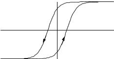
The relationship between B and H in ferromagnetic substances is nonlinear and is characterized by a BH curve. A typical curve is shown in Fig. 8.24. The fact that the curves for increasing and decreasing H do not coincide is called hysteresis. The arrows show the direction in which H changes on each branch of the curve. Saturation takes place beyond points W and Y . The value of M saturates and B = µ0 (Msaturated + H) . When H = 0 there is a remanent magnetic field (points X and Z). If the temperature of the sample is raised above a critical temperature called the Curie temperature, the magnetism is destroyed.
8.8.2Measuring Magnetic Properties in People
Several kinds of measurements can be based on magnetic e ects in materials. A common component of dust inhaled by miners and industrial workers is magnetite, Fe3O4, which is ferrimagnetic. By placing the thorax in a fixed magnetic field for a few seconds, the particles can be aligned. The field is turned o and the remanent field measured. The use of magnetopneumography in occupational health is described by Stroink (1985). Cohen et al. (1984) have modeled the process by which the particles are magnetized, as well as the relaxation process by which the magnetization disappears after the external field is removed. Relaxation curves are used to estimate intracellular viscosity and the motility of macrophages (scavenger white cells) in the alveoli [Stahlhofen and Moller (1993)].
The magnetic susceptibility of blood and myocardium is di erent from the susceptibility of surrounding lung tissue. An externally applied magnetic field induces a field that changes as the volume of the heart changes. It can